Amortized Analysis

Some structures cannot be made cheap on every single call, but can be made cheap on average over any run. A dynamic array occasionally has to grow: allocate a bigger buffer, copy everything into it. That one call is expensive. But if growth happens rarely enough, and the cost of each growth is proportional to how much cheap work already happened since the last one, the expensive calls pay for themselves.

Amortized analysis makes that intuition precise, without appealing to probability. "Average case" describes a distribution over inputs and can be defeated by an adversarial one. "Amortized" describes a worst-case sequence of operations and cannot be defeated by any input — the bound holds for every possible sequence, not just typical ones. That distinction is the entire point of the technique: it is a worst-case guarantee stated over time instead of over a single call.

There are three standard ways to prove an amortized bound, and they prove the same number by different routes. Aggregate analysis sums the total cost directly. The accounting method assigns each operation a fixed "charge" and lets cheap operations save up credit for expensive ones. The potential method tracks a function of the structure's state and charges each operation for how much that function rises. Which one to reach for depends on the structure — aggregate suffices when the total is easy to sum directly, but accounting and potential generalise better to structures with several operation types.

Core Concepts

Term	Meaning
Aggregate method	Sum the total cost of n operations, divide by n
Accounting method	Each operation pays a fixed amortized charge; overpayment becomes stored credit, never negative
Potential method	Φ(state) tracks "banked work"; amortized cost = actual cost + ΔΦ
Amortized ≠ average	Amortized bounds every sequence, worst case; average bounds a distribution of inputs
α(n), inverse Ackermann	Grows so slowly it is effectively constant for any n reachable in practice

Mechanism

Most appends cost 1. The rare resize at each power of two costs the whole array's worth of copies — but averaged over any run, the cost per append never exceeds 3.

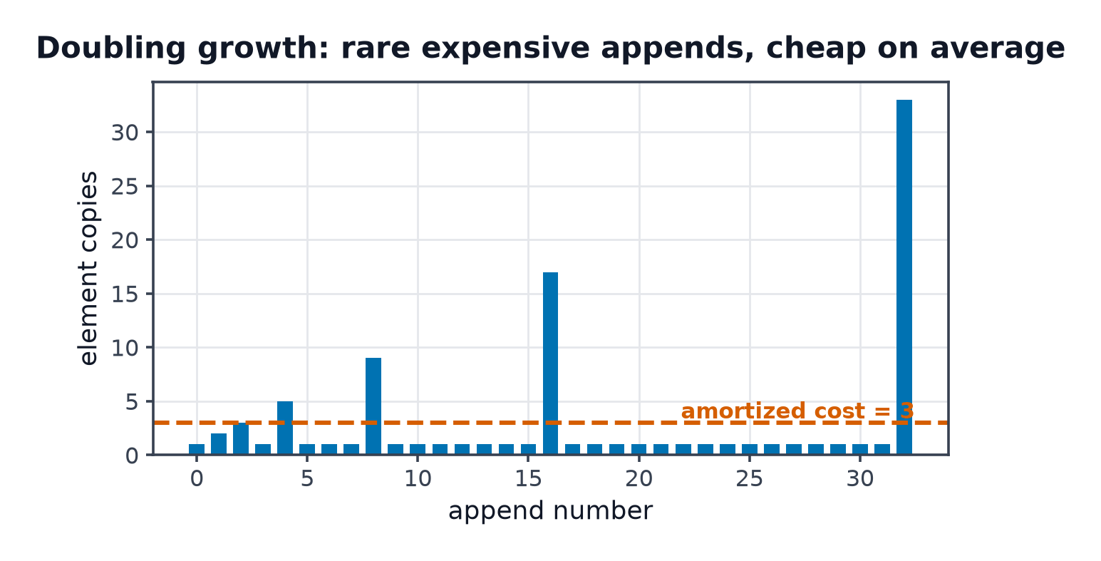
Aggregate: the doubling dynamic array

Growing a dynamic array by doubling means resizes happen only at sizes 1, 2, 4, 8, …. Trace 16 appends, each row the individual cost and the running total:

append #    resize?      copy cost      running total    running total / n
   1        yes (0→1)        1                1               1.00
   2        yes (1→2)        1                2               1.00
   3        yes (2→4)        2                4               1.33
   4        no               0                4               1.00
   5        yes (4→8)        4                8               1.60
   6        no               0                8               1.33
   7        no               0                8               1.14
   8        no               0                8               1.00
   9        yes (8→16)       8               16               1.78
  10..16    no (7 appends)   0               16               1.00

Total cost through append 16: each append itself costs 1 (writing the element) plus the occasional copy. Copies across all 16 appends sum to 1 + 2 + 4 + 8 = 15 — always less than 2n because 1 + 2 + 4 + … + n < 2n for a geometric series. Sixteen appends, at most 16 + 15 = 31 total units of work, or under 2 per append — $O(1)$ amortized, even though append 9 alone cost 8 units.

Accounting: charge 3, bank the rest

Charge every append a fixed fee of 3 "coins", spend 1 immediately (writing the new element), and bank 2. When a resize of size k fires, it must move all k existing elements — pay for that move entirely out of banked coins. Because the array last resized at size k/2, exactly k/2 appends have happened since, each banking 2 coins: k/2 × 2 = k coins available, exactly enough to move k elements. The balance never goes negative, which is the accounting method's proof obligation — so a flat charge of $O(1)$ per append is a valid amortized bound.

Potential: Φ = 2·(size − capacity/2)

Define Φ as twice the gap between the array's current size and half its capacity — zero right after a resize, maximal right before the next one. A cheap append raises size by 1, raising Φ by 2, so amortized cost = actual cost (1) + ΔΦ (2) = 3. A resize's actual cost is proportional to the array's size, but Φ drops by exactly that much (the gap resets to zero), cancelling the spike — so amortized cost is $O(1)$ there too. All three methods land on the same constant; they differ only in how the bookkeeping is carried out.

A second worked example: the binary counter

A k-bit binary counter starts at 0; each increment flips the trailing run of 1-bits to 0 and the next 0-bit to 1. Flipping a bit is the unit of cost. Incrementing 0111 to 1000 flips 4 bits — expensive — but most increments flip only 1 or 2. Trace the first eight increments, bits flipped each time:

counter   flips this increment    running total flips
0000        —                        0
0001        1                        1
0010        2                        3
0011        1                        4
0100        3                        7
0101        1                        8
0110        2                       10
0111        1                       11
1000        4                       15

Aggregate: bit 0 flips every increment (8 times in 8 increments), bit 1 flips every other increment (4 times), bit 2 every fourth (2 times), bit 3 every eighth (1 time) — total 8 + 4 + 2 + 1 = 15, matching the trace, and bounded above by 2n for n increments, since it is a geometric series identical in shape to the dynamic array's copy count. $O(1)$ amortized per increment, even though flipping 0111→1000 alone costs 4 — the same "rare expensive operation paid for by prior cheap ones" pattern as doubling, proven by the same aggregate argument.

Union-find's α(n): stated, not derived

Union-find with union-by-rank and path compression gives $O(α(n))$ amortized per operation, where α is the inverse Ackermann function — it grows so slowly that α(n) < 5 for any n representable in this universe. The proof is a separate, lengthy potential-function argument over the rank forest and is stated here rather than derived; see Union-Find for the structure itself and Tarjan's original potential-based proof, cited below.

Python

def doubling_costs(n):
    """Copy cost of each append into a doubling array; returns (per-append costs, total)."""
    costs = []
    capacity = 0
    for size in range(1, n + 1):
        if size > capacity:
            capacity = max(1, capacity * 2)
            costs.append(size - 1)   # copy everything that existed before this append
        else:
            costs.append(0)
    return costs, sum(costs) + n     # + n: the write itself, one unit per append


costs, total = doubling_costs(16)
assert costs == [0, 1, 2, 0, 4, 0, 0, 0, 8, 0, 0, 0, 0, 0, 0, 0]
assert total == 31
assert total / 16 < 2.0          # amortized O(1): under 2 units of work per append

C++

#include <cassert>
#include <vector>

std::vector<long long> doubling_costs(int n) {
    std::vector<long long> costs;
    long long capacity = 0;
    for (int size = 1; size <= n; ++size) {
        if (size > capacity) {
            capacity = std::max<long long>(1, capacity * 2);
            costs.push_back(size - 1);
        } else {
            costs.push_back(0);
        }
    }
    return costs;
}

Practical Usage

std::vector::push_back is documented as amortized constant time — "the complexity is amortized constant" [vector.modifiers] — and Python's list.append carries the same guarantee as a CPython implementation detail (the CPython source over-allocates by a growth factor near 1.125, not 2, but the amortized argument is identical). Neither language's list exposes a way to force pre-growth in the general case; C++'s vector::reserve does, which is the fix when p99 latency, not just throughput, matters.

The same reasoning applies wherever a rare expensive step is proportional to the cheap work since the last one: table-doubling hash maps, a binary counter's carry chain (incrementing n times flips $O(n)$ bits total, not $O(n \log n)$), and splay trees, whose $O(\log n)$ amortized bound per operation comes from a potential function over subtree sizes.

Edge Cases & Pitfalls

• Quoting amortized $O(1)$ as a per-call latency guarantee. It is not one. A single append can still trigger a full copy; a real-time path that cannot tolerate that spike wants reserve or a structure with a genuine worst-case bound, not an amortized one.
• Growing by a fixed amount instead of a fixed factor. Growing capacity by +1 each time (rather than ×2) makes total copying cost 1 + 2 + … + n = Θ(n²), i.e. $O(n)$ amortized per append, not $O(1)$ — resizes never get rarer relative to the work already banked.
• Confusing amortized with average case. Average case is a claim about a distribution of inputs and an adversary can construct a bad one. Amortized is a claim about worst-case totals across any sequence — there is no adversarial input that breaks it.
• Forgetting the credit can only be spent once. In the accounting method, a common bug is charging the same banked coin to two different future operations; the proof only holds if every unit of credit is spent exactly once, at the operation that needed it.

Comparisons

	Amortized	Worst-case	Average-case
What it bounds	Any sequence's total, divided by n	Every single operation	A distribution over inputs
Defeated by	Nothing — holds for all sequences	Nothing — holds always	An adversarial input
Example	Dynamic array append: $O(1)$	Balanced-tree lookup: $O(\log n)$	Randomised quicksort: $O(n \log n)$
Latency-sensitive systems	Risky — one call can spike	Safe	Risky — same reason

Recall

InvariantAn amortized bound is a guarantee on the total cost of any sequence of n operations, divided by n — never a claim about any single operation.

Costs

dynamic array append, doubling (amortized)$O(1)$

dynamic array append, doubling (worst, single op)$O(n)$

union-find union/find with union-by-rank + path compression (amortized)$O(\alpha (n))$

binary counter increment (amortized)$O(1)$

binary counter increment (worst, single op)$O(\log n)$

Reach for itA structure where most operations are cheap and a few are expensive, and the expensive ones become rarer exactly in proportion to how much cheap work preceded them.

TrapReporting the amortized bound as if it bounded every call — a single append can still be $O(n)$, and a real-time or interactive path judged on tail latency will see that cost directly.

References

• Cormen, Leiserson, Rivest & Stein, Introduction to Algorithms, 4th ed., Ch. 16 — "Amortized Analysis", covering all three methods (aggregate, accounting, potential) with the dynamic-table and binary-counter examples used here.
• Tarjan, R. E., "Amortized Computational Complexity" (1985) — the original potential-function proof that union-find with union-by-rank and path compression is $O(α(n))$ amortized per operation.
• [vector.modifiers] — the C++ standard's own wording for push_back's amortized constant complexity.
• CPython listobject.c — the over-allocation growth pattern behind list.append's amortized $O(1)$, an implementation detail rather than a language guarantee.

Related Pages

• Union-Find — the structure whose $O(α(n))$ amortized bound this page states rather than proves.
• Common Complexities — where amortized cost sits among the other growth classes met day to day.
• Recurrences & the Master Theorem — the other main tool for bounding recursive and iterative costs, used when the cost is not amortized but recursive.
• Arrays & Dynamic Arrays — the doubling-array mechanics this page analyses, described as a structure rather than as a cost argument.