Big-O Notation

Overview

Big-O describes an upper bound on growth. Saying an algorithm is O(n²) claims that beyond some input size, its cost is at most a constant multiple of n² — never that it is n², and never anything at all about small inputs.

That "beyond some input size" clause is the part most explanations skip, and it is the part that makes the notation work. It is what licenses throwing away constants and lower-order terms, because for large enough n those genuinely stop mattering.

Core Concepts

Term	Meaning	Everyday reading
O(f)	Grows no faster than f	Upper bound — "at worst this"
Ω(f)	Grows no slower than f	Lower bound — "at best this"
Θ(f)	Bounded above and below by f	Tight bound — "exactly this rate"
o(f)	Grows strictly slower than f	Strict upper bound

Informal usage almost always says "O" where "Θ" is meant. Saying mergesort is O(n log n) is true but weak — it is also O(n³), since that is a valid upper bound too. Saying mergesort is Θ(n log n) is the stronger, more useful claim. In practice, when someone says "quicksort is O(n log n) on average", read Θ.

Architecture / Mechanism

The formal definition, and what it is doing

f(n) = O(g(n)) means: there exist positive constants c and n₀ such that for all n ≥ n₀,

f(n) ≤ c · g(n)

Beyond the crossover point (x₀), c·g(n) stays above f(n) forever. Everything to the left of it is explicitly outside the claim. Wikimedia Commons, Public domain

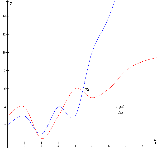
The two knobs are what make the abstraction useful. Because you may pick any constant c, a factor of 100 in speed cannot change the classification. Because you may pick any starting point n₀, behaviour on small inputs cannot change it either.

Why constants and lower-order terms vanish

Given f(n) = 3n² + 500n + 90000:

n	3n²	500n	90000	Which dominates
10	300	5,000	90,000	the constant
100	30,000	50,000	90,000	still the constant
1,000	3,000,000	500,000	90,000	n²
100,000	3×10¹⁰	5×10⁷	90,000	n², overwhelmingly

So f(n) = O(n²). The other terms are not wrong, they simply stop being the story. Note also that at n = 100 this function is dominated by a constant — a real reminder that asymptotic claims say nothing about the range you might actually be operating in.

Reading complexity off code

The mechanical rules cover most cases:

# O(1) — the work does not depend on n
def first(items):
    return items[0]

# O(n) — one pass
def total(items):
    acc = 0
    for x in items:          # n iterations
        acc += x             # O(1) each
    return acc

# O(n²) — nested loops over the same input
def has_duplicate(items):
    for i in range(len(items)):          # n
        for j in range(i + 1, len(items)):  # up to n
            if items[i] == items[j]:
                return True
    return False

# O(log n) — the search space halves each step
def count_halvings(n):
    steps = 0
    while n > 1:
        n //= 2
        steps += 1
    return steps

• Sequential blocks add, and the larger wins: O(n) + O(n²) = O(n²).
• Nested loops multiply: a loop of n containing a loop of m is O(n·m).
• Halving (or doubling) the problem each step is logarithmic — that is what a logarithm counts.

Edge Cases & Pitfalls

The variable you dropped is still in there

O(n) is meaningless until you say what n counts. Two common traps:

• Two different inputs. Comparing every element of one list against another is O(n·m), not O(n²) — and if m is tiny and fixed, it is effectively O(n).
• Cost per operation. Summing a list of integers is O(n). Concatenating a list of strings with += in a loop is O(n²), because each concatenation copies everything accumulated so far. The loop looks identical; the per-iteration cost is not O(1).

• O(n²) is not always worse than O(n log n). With a large constant hidden inside, the "better" algorithm can lose on real input sizes. This is exactly why production sorts switch to insertion sort below a threshold of ~16 elements.
• Best/average/worst are separate questions from O/Ω/Θ, though the two are constantly conflated. You can state a Θ bound on the worst case, or an O bound on the average case; the notation and the case being analysed are independent choices.
• Amortized is not average. See Common Complexities — an amortized bound is a guarantee over any sequence of operations, not a probabilistic statement.

Comparisons

Claim	Says	Does not say
"Quicksort is O(n²)"	Its worst case is quadratic	Anything about the typical case, which is n log n
"Lookup is O(1)"	Cost does not grow with the collection	That it is fast — a hash may be expensive
"This is faster, it's O(n) not O(n log n)"	It scales better	That it wins at your n

References

• Cormen, Leiserson, Rivest & Stein, Introduction to Algorithms, Ch. 3 — "Characterizing Running Times", the formal treatment of O, Ω and Θ.
• Knuth, The Art of Computer Programming, Vol. 1, §1.2.11 — the origin of the notation's use in this field.

Books & Videos

• Big-O Cheat Sheet — complexity tables for the common structures and sorts, useful as a lookup rather than a lesson.

Related Pages

• Common Complexities — the growth classes you will actually meet, plus amortized and space analysis.
• Sorting Algorithms — where these bounds get their most familiar workout.