Balanced Trees

A binary search tree is $O(\log n)$ only while it stays short, and nothing in the plain insertion algorithm keeps it short. A self-balancing tree restores a height bound after every modification, converting the average case into a worst-case guarantee.

The mechanism is always a rotation — a local, constant-time pointer rearrangement that changes the tree's shape without changing its in-order sequence. AVL, red-black, and B-trees differ only in when a rotation fires and how strict the height bound it enforces is.

Core Concepts

Structure	Balance invariant	Height bound	Typical use
AVL tree	Subtree heights differ by ≤ 1 at every node	≤ 1.44 log₂ n	Read-heavy workloads
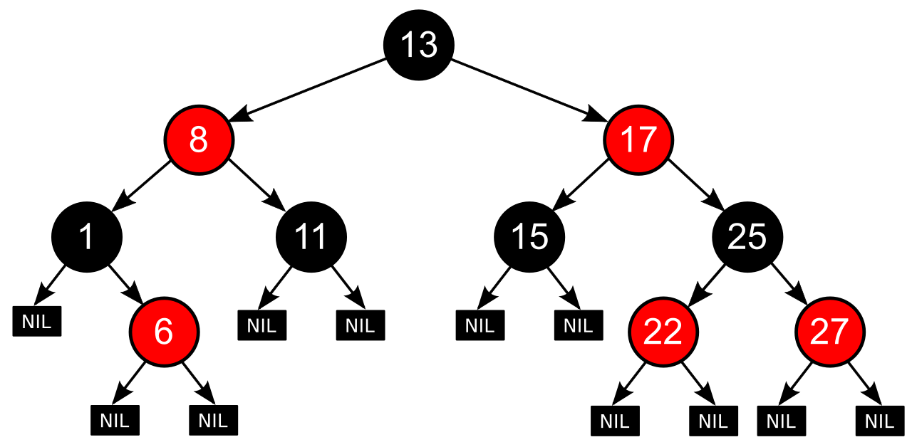
Red-black tree	No red node has a red child; equal black-depth on all root-to-leaf paths	≤ 2 log₂(n+1)	Language library maps/sets
B-tree / B+ tree	All leaves at the same depth; nodes hold many keys	log_B n	Databases, filesystems
Trie	Not a search tree — position encodes the key, not comparison	Length of the key	Prefix queries; see Tries

Mechanism

The rotation, in isolation

A rotation swaps a parent and child while re-parenting one subtree, preserving the BST ordering — the in-order sequence A x B y C is identical before and after:

      y                               x
     / \        right rotation       / \
    x   C       ───────────────>    A   y
   / \          <───────────────       / \
  A   B          left rotation        B   C

In-order before:  A x B y C
In-order after:   A x B y C      (identical — only the shape changed)

AVL: the four imbalance shapes, each shown before and after

An AVL node's balance factor is height(left) − height(right); a rotation fires the moment any node's balance factor reaches ±2, and there are exactly four shapes that trigger it, each with a fixed fix:

Case LL — inserting into the left subtree of a left child. Insert 30, 20, 10 in that order:

before (30's balance factor = +2)      after: single RIGHT rotation at 30

      30                                    20
     /                                     /  \
    20              ────────────>        10    30
   /
  10

Case RR — the mirror. Insert 10, 20, 30 in that order:

before (10's balance factor = -2)      after: single LEFT rotation at 10

  10                                        20
    \                                      /  \
     20            ────────────>         10    30
       \
        30

Case LR — inserting into the right subtree of a left child. Insert 30, 10, 20:

before (a single rotation at 30 won't fix this — 10 leans right, not left)

  30                                    30
 /                                     /
10       step 1: LEFT rot. at 10 ->   20       step 2: RIGHT rot. at 30 ->    20
  \                                  /                                      /  \
   20                              10                                     10   30

Case RL — the mirror. Insert 10, 30, 20:

before (a single rotation at 10 won't fix this — 30 leans left, not right)

10                                    10
  \                                     \
   30     step 1: RIGHT rot. at 30 ->    20      step 2: LEFT rot. at 10 ->    20
  /                                        \                                 /  \
 20                                         30                              10   30

LL and RR cost one rotation; LR and RL cost two, because the first rotation only reshapes the child into a straight line — the second one is the actual fix. Either way the cost per insertion is $O(1)$ rotations, found in $O(\log n)$ worst case by walking back up from the inserted leaf (Sedgewick & Wayne, 4th ed., §3.3; CLRS 4th ed. treats AVL as an exercise in Ch. 13, using red-black trees as the worked example instead).

The same LL/RR/LR/RL fix-ups traced above, animated across a longer sequence of insertions — each rotation fires the instant a balance factor reaches ±2. Wikimedia Commons, CC BY-SA 4.0

All four traced sequences above happen to converge on the same three-node tree, which makes them a convenient self-check for an implementation:

Python

class N:
    def __init__(self, v): self.v, self.l, self.r, self.h = v, None, None, 1

def h(n): return n.h if n else 0
def bf(n): return h(n.l) - h(n.r)
def fix(n): n.h = 1 + max(h(n.l), h(n.r))

def rot_right(y):
    x = y.l; y.l, x.r = x.r, y; fix(y); fix(x); return x

def rot_left(x):
    y = x.r; x.r, y.l = y.l, x; fix(x); fix(y); return y

def insert(n, v):
    if n is None: return N(v)
    if v < n.v: n.l = insert(n.l, v)
    else: n.r = insert(n.r, v)
    fix(n)
    b = bf(n)
    if b > 1 and v < n.l.v: return rot_right(n)                    # LL
    if b < -1 and v > n.r.v: return rot_left(n)                    # RR
    if b > 1: n.l = rot_left(n.l); return rot_right(n)             # LR
    if b < -1: n.r = rot_right(n.r); return rot_left(n)            # RL
    return n

for seq in ([30, 20, 10], [10, 20, 30], [30, 10, 20], [10, 30, 20]):
    root = None
    for v in seq: root = insert(root, v)
    assert root.v == 20 and root.l.v == 10 and root.r.v == 30      # all four cases converge

C++

#include <algorithm>
#include <cassert>
#include <vector>

struct N { int v, ht = 1; N *l = nullptr, *r = nullptr; explicit N(int x) : v(x) {} };

int h(N* n) { return n ? n->ht : 0; }
int bf(N* n) { return n ? h(n->l) - h(n->r) : 0; }
void fix(N* n) { n->ht = 1 + std::max(h(n->l), h(n->r)); }

N* rot_right(N* y) { N* x = y->l; y->l = x->r; x->r = y; fix(y); fix(x); return x; }
N* rot_left(N* x) { N* y = x->r; x->r = y->l; y->l = x; fix(x); fix(y); return y; }

N* insert(N* n, int v) {
    if (!n) return new N(v);
    if (v < n->v) n->l = insert(n->l, v); else n->r = insert(n->r, v);
    fix(n);
    int b = bf(n);
    if (b > 1 && v < n->l->v) return rot_right(n);                       // LL
    if (b < -1 && v > n->r->v) return rot_left(n);                       // RR
    if (b > 1) { n->l = rot_left(n->l); return rot_right(n); }           // LR
    if (b < -1) { n->r = rot_right(n->r); return rot_left(n); }          // RL
    return n;
}

void check_all_four_cases() {
    std::vector<std::vector<int>> cases{{30,20,10}, {10,20,30}, {30,10,20}, {10,30,20}};
    for (auto& seq : cases) {
        N* root = nullptr;
        for (int v : seq) root = insert(root, v);
        assert(root->v == 20 && root->l->v == 10 && root->r->v == 30);   // all four converge
    }
}

Red-black: the same rotation, plus a colour that avoids most of them

A red-black tree tolerates a looser invariant — no red node has a red child, and every root-to-leaf path has the same number of black nodes — which needs fewer rotations per fix-up, at the cost of a taller tree. Inserting 10, 20, 30 in that order (mirroring the RR case above) creates a red-red violation the moment 30 is added as 20's red child, with no black uncle to recolour around:

before (10 black, 20 red, 30 red — a straight red-red violation, RR shape)

   10(B)
     \
      20(R)
        \
         30(R)

after: single LEFT rotation at 10, then recolour — 20 becomes black, 10 and 30 become red

      20(B)
     /    \
   10(R)  30(R)

The rotation is identical to the AVL case; what red-black adds is that a differently shaped violation (an uncle that is red rather than absent) is fixed by recolouring alone, with no rotation at all — which is why red-black trees rotate less often in practice than AVL trees, at ≤ 3 rotations per deletion regardless of tree size (CLRS 4th ed. §13.4, Lemma 13.4).

Every root-to-leaf path passes through the same number of black nodes; red nodes never have a red child — the invariant that bounds height at 2 log₂(n+1) without AVL's stricter balance factor. Wikimedia Commons, CC BY-SA 3.0

	AVL	Red-black
Height (worst case)	≤ 1.44 log₂ n	≤ 2 log₂(n+1)
Lookup (worst case)	Faster — shorter tree	Slightly slower
Insert / delete	More rotations	Fewer — ≤ 3 per delete
Used by	Some in-memory indexes	C++ std::map/std::set, Linux CFS scheduler

Red-black won the standard-library slot almost everywhere: mixed read/write workloads are the common case, and a small constant worst-case deletion cost beats a shorter tree that costs more to maintain.

B-trees: sized for disk, and the fanout arithmetic that makes it work

A binary tree node holds one key and decides one of two directions. When a node lives on storage and reading it costs an entire page, deciding one bit per page fetched is a catastrophic ratio. A B-tree sizes each node to exactly one page and packs it with as many keys as fit, so a single I/O narrows the search hundreds of ways instead of two.

Work the fanout for a realistic page: a 4 KiB (4,096-byte) page, an 8-byte key (a 64-bit integer or a row pointer), and an 8-byte child pointer. A node with $m$ children holds $m - 1$ keys and $m$ pointers:

node size = (m - 1) x 8 bytes(key) + m x 8 bytes(pointer)  <=  4,096 bytes
          = 8m - 8 + 8m  <=  4,096
          = 16m          <=  4,104
          = m            <=  256.5   ->   m = 256 children, 255 keys per node

A tree of height 3 (root, one internal level, leaves) then indexes up to $256^2$ leaf nodes, each holding 255 keys — on the order of $256^2 \times 255 \approx 16.7$ million keys reachable in exactly three page reads, worst case, versus $\log_2(16{,}700{,}000) \approx 24$ page reads for a binary tree over the same key count. This is the entire argument for B-trees: fanout trades comparisons (free, in-memory) for page reads (expensive, on disk), and a wider node makes that trade far more aggressively than a binary one (CLRS 4th ed. Ch. 18, "B-Trees", develops this bound in general form as a function of the minimum degree $t$).

B+ trees, the variant databases actually use, additionally keep all values in the leaves and link the leaves together in a linked list, making a range scan a sequential walk instead of a repeated root-down descent per key.

Practical Usage

Language	Ordered map	Underlying structure
C++	std::map, std::set	Red-black tree, in every major implementation
Python	(none built in)	Use sortedcontainers, or keep a sorted list + bisect
Rust	BTreeMap, BTreeSet	B-tree — chosen for cache behaviour, in memory
Go	(none built in)	Sort a slice, or use a third-party tree

What "std::map is a red-black tree" actually rests on

The C++ standard names no data structure for std::map, only complexity: $O(\log n)$ worst case for insertion, lookup, and erasure (cppreference). That bound is only achievable with a balanced tree, and every major implementation (libstdc++, libc++, MSVC) happens to use a red-black tree to meet it — true everywhere in practice, but an implementation choice, not a standard requirement.

Rust's BTreeMap choice is the interesting one

BTreeMap uses a B-tree in memory, one level down the hierarchy from disk — here the "page" is a cache line, and packing many keys per node turns one cache miss into a many-way search step instead of two, per the Rust documentation's own rationale.

Python's dict is not a tree at all — it is a hash table that has preserved insertion order since 3.7 (a property of iteration order, not of key order). Asking it for keys in sorted order, or for a range query, is not a slower version of what dict does — it is a query dict structurally cannot answer, which is the actual reason to reach for a balanced tree instead of "just using a dict and sorting."

Edge Cases & Pitfalls

• Do not implement one unless you must. Red-black deletion has many cases (CLRS 4th ed. §13.4 lists six) and is genuinely easy to get subtly wrong. Every mainstream standard library ships a correct one.
• A balanced tree is not a hash table. If you never need ordering, ranges, or a worst-case bound, a hash table is faster and simpler — see the comparison table there.
• "Balanced" bounds height, not shape. Two trees holding the same keys can differ completely in structure depending on insertion order; only the height bound is guaranteed, not the tree itself.
• B-tree fanout is not free. Wider nodes mean more keys to scan within a node once loaded — real implementations binary-search or use SIMD within a node, so "256 comparisons per level" overstates the real per-level cost implied by the arithmetic above.
• Confusing B-tree "order" definitions across sources. Order as max children, as max keys, or as the minimum degree $t$ (CLRS's convention) all appear in different texts — check which one a source uses before comparing numbers across them.

Comparisons

	Trees & BSTs (unbalanced)	Balanced tree (AVL/RB)	B-tree	Hash table
Search / insert / delete	$O(\log n)$ avg, $O(n)$ worst	$O(\log n)$ worst	$O(\log_B n)$ worst	$O(1)$ expected
Sorted iteration	Yes	Yes	Yes	No
Optimised for	Nothing in particular	In-memory comparisons	Page/block I/O	Exact-key lookup
Rotations needed	n/a	Yes, on every fix-up	No — splits/merges instead	n/a

Recall

InvariantA rotation is a constant-time, order-preserving reshape; every self-balancing scheme is that one primitive applied under a different trigger and a different strictness of height bound.

Costs

AVL/red-black search, insert, delete (worst)$O(\log n)$

rotations per AVL insert (worst)$O(1)$, found via an $O(\log n)$ walk

rotations per red-black delete (worst)at most 3

B-tree search, insert, delete (worst)$O({\log }_{B}n)$

Reach for itYou need sorted iteration, range queries, or a worst-case bound that a plain BST or hash table cannot give you.

TrapAssuming std::map being 'a red-black tree' is a language guarantee — it's an implementation detail that happens to be universal, backed only by the complexity requirement in the standard, not a named data structure.

References

• Cormen, Leiserson, Rivest & Stein, Introduction to Algorithms, 4th ed., Ch. 13 ("Red-Black Trees") and Ch. 18 ("B-Trees") — the fix-up case analysis and the general fanout bound in terms of minimum degree $t$.
• Sedgewick & Wayne, Algorithms, 4th ed., §3.3 ("Balanced Search Trees") — AVL and red-black-like 2-3 trees developed with the rotation cases illustrated step by step.
• cppreference, std::map — the complexity requirements every implementation's red-black tree exists to satisfy.
• Rust BTreeMap documentation — the standard library's own rationale for using a B-tree in memory.

Related Pages

• Trees & Binary Search Trees — the unbalanced base case and why it degenerates.
• Tries — a different way to bound depth, by keying on position instead of comparison.
• Hash Tables — the unordered alternative, and why dict cannot replace a tree.
• Indexing & Storage Engines — B+ trees under real query loads.