Graphs

A graph is a set of vertices and a set of edges connecting them. That is nearly no structure at all, which is precisely why it models so much: road networks, social connections, package dependencies, web links, state machines, and the call graph of the program you are reading this in.

Trees and linked lists are special cases — a tree is a connected graph with no cycles, a linked list a tree where every node has one child.

An undirected graph on six vertices. Note vertex 6 hanging off a single edge — removing it disconnects the graph, which makes it a bridge. Wikimedia Commons, Public domain

Core Concepts

Term	Meaning
Vertex (node)	An entity
Edge	A relationship between two vertices
Directed / undirected	Whether edges have a direction (follower vs. friendship)
Weighted	Edges carry a cost — distance, latency, price
Degree	Number of edges at a vertex (in-degree/out-degree when directed)
Path	A sequence of vertices joined by edges
Cycle	A path returning to its start
Connected	Every vertex reachable from every other
DAG	Directed acyclic graph — directed, no cycles
Dense / sparse	E close to $V^2$ / E close to V

DAGs deserve their own line

A DAG. Because no path returns to where it started, the vertices can always be laid out so that every arrow points forward — that ordering is a topological sort. Wikimedia Commons, Public domain

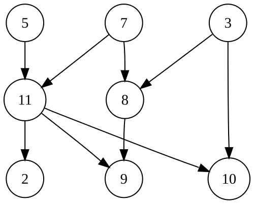
Acyclicity is what makes dependency resolution, build systems, task scheduling and spreadsheet recalculation possible: it guarantees a valid order exists. A cycle in any of those is precisely the error condition ("circular dependency"). See Topological Sort.

Mechanism

The two representations

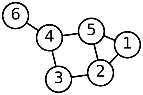
Adjacency list — each vertex stores its neighbours:

Python

graph = {
    1: [2, 5],
    2: [1, 3, 5],
    3: [2, 4],
    4: [3, 5, 6],
    5: [1, 2, 4],
    6: [4],
}
# Weighted: store (neighbour, weight) pairs
weighted = {
    1: [(2, 7), (5, 3)],
    2: [(1, 7), (5, 1)],
    # ... one entry per vertex, same shape as the unweighted graph above
}

C++

#include <array>
#include <unordered_map>
#include <utility>
#include <vector>

std::unordered_map<int, std::vector<int>> graph{
    {1, {2, 5}},
    {2, {1, 3, 5}},
    {3, {2, 4}},
    {4, {3, 5, 6}},
    {5, {1, 2, 4}},
    {6, {4}},
};
// Weighted: store (neighbour, weight) pairs
std::unordered_map<int, std::vector<std::pair<int, int>>> weighted{
    {1, {{2, 7}, {5, 3}}},
    // ...
};

Adjacency matrix — a V×V grid where m[i][j] marks an edge:

Python

#      1  2  3  4  5  6
m = [[0, 1, 0, 0, 1, 0],   # 1
     [1, 0, 1, 0, 1, 0],   # 2
     [0, 1, 0, 1, 0, 0],   # 3
     [0, 0, 1, 0, 1, 1],   # 4
     [1, 1, 0, 1, 0, 0],   # 5
     [0, 0, 0, 1, 0, 0]]   # 6

C++

//                                    1  2  3  4  5  6
std::array<std::array<int, 6>, 6> m{{{0, 1, 0, 0, 1, 0},    // 1
                                     {1, 0, 1, 0, 1, 0},    // 2
                                     {0, 1, 0, 1, 0, 0},    // 3
                                     {0, 0, 1, 0, 1, 1},    // 4
                                     {1, 1, 0, 1, 0, 0},    // 5
                                     {0, 0, 0, 1, 0, 0}}};  // 6

	Adjacency list	Adjacency matrix
Space	$O(V + E)$	$O(V^2)$
Is there an edge u→v?	$O(degree(u))$	$O(1)$
Iterate u's neighbours	$O(degree(u))$	$O(V)$ — scans empty cells too
Add an edge	$O(1)$	$O(1)$
Best for	Sparse graphs — nearly all real ones	Dense graphs; matrix algorithms

Default to the adjacency list

Real graphs are overwhelmingly sparse. A social network with a million users and a hundred friends each has $10^8$ edges — an adjacency list holds that comfortably, while the matrix needs $10^{12}$ cells, 99.99% of them zero. Reach for a matrix only when the graph is genuinely dense, or when an algorithm wants matrix form (Floyd–Warshall, spectral methods).

One weighted graph, three representations, traced

Six vertices A B C D E F, nine weighted undirected edges: A–B 4, A–C 2, B–C 1, B–D 5, C–D 8, C–E 10, D–E 2, D–F 6, E–F 3. Building all three representations from the same edge list, with an approximate byte cost for a compact fixed-width layout (1 byte per vertex id, 4 bytes per integer weight, no per-object/pointer overhead — real language containers add more):

adjacency list (each undirected edge stored once per endpoint — 18 directed entries total)
  A: [(B,4), (C,2)]
  B: [(A,4), (C,1), (D,5)]
  C: [(A,2), (B,1), (D,8), (E,10)]
  D: [(B,5), (C,8), (E,2), (F,6)]
  E: [(C,10), (D,2), (F,3)]
  F: [(D,6), (E,3)]
  cost: 18 entries x (1 byte id + 4 byte weight) = 90 bytes         — O(V + E)

adjacency matrix (6x6, one 4-byte weight per cell, 0 meaning "no edge")
      A   B   C   D   E   F
  A [ 0,  4,  2,  0,  0,  0]
  B [ 4,  0,  1,  5,  0,  0]
  C [ 2,  1,  0,  8, 10,  0]
  D [ 0,  5,  8,  0,  2,  6]
  E [ 0,  0, 10,  2,  0,  3]
  F [ 0,  0,  0,  6,  3,  0]
  cost: 36 cells x 4 bytes = 144 bytes                              — O(V^2)

edge list (each undirected edge stored exactly once)
  [(A,B,4), (A,C,2), (B,C,1), (B,D,5), (C,D,8), (C,E,10), (D,E,2), (D,F,6), (E,F,3)]
  cost: 9 entries x (2 x 1 byte id + 4 byte weight) = 54 bytes       — O(E)

Three representations of the same nine edges span 90, 144 and 54 bytes here — a small enough graph that the difference looks minor, but the matrix's $V^2$ term dominates at scale exactly as the tip above argues. The edge list is smallest because it is the only one of the three that never repeats a fact: each edge appears once, where the other two either duplicate it (undirected list) or reserve space for every non-edge (matrix).

Python

edges = [("A","B",4), ("A","C",2), ("B","C",1), ("B","D",5), ("C","D",8),
         ("C","E",10), ("D","E",2), ("D","F",6), ("E","F",3)]

adj = {v: [] for v in "ABCDEF"}
for u, v, w in edges:
    adj[u].append((v, w))
    adj[v].append((u, w))
assert adj["A"] == [("B", 4), ("C", 2)]
assert len(adj["C"]) == 4      # C touches A, B, D, E

idx = {v: i for i, v in enumerate("ABCDEF")}
matrix = [[0] * 6 for _ in range(6)]
for u, v, w in edges:
    matrix[idx[u]][idx[v]] = w
    matrix[idx[v]][idx[u]] = w
assert matrix[idx["A"]][idx["B"]] == 4
assert matrix[idx["D"]][idx["F"]] == 6

assert len(edges) == 9         # the edge list: exactly one entry per edge

C++

struct WeightedEdge { char u, v; int w; };

std::vector<WeightedEdge> edges{
    {'A','B',4}, {'A','C',2}, {'B','C',1}, {'B','D',5}, {'C','D',8},
    {'C','E',10}, {'D','E',2}, {'D','F',6}, {'E','F',3},
};

int index_of(char v) { return v - 'A'; }

void build_representations() {
    std::unordered_map<char, std::vector<std::pair<char, int>>> adj;
    std::array<std::array<int, 6>, 6> matrix{};
    for (const auto& e : edges) {
        adj[e.u].push_back({e.v, e.w});
        adj[e.v].push_back({e.u, e.w});
        matrix[index_of(e.u)][index_of(e.v)] = e.w;
        matrix[index_of(e.v)][index_of(e.u)] = e.w;
    }
}

Practical Usage

Python

# doc:no-run
from collections import defaultdict

# Building an undirected graph from an edge list
graph = defaultdict(list)
for u, v in edges:
    graph[u].append(v)
    graph[v].append(u)      # omit this line for a directed graph

# Degree of a vertex
len(graph[v])

C++

// doc:no-run
// Building an undirected graph from an edge list
std::unordered_map<int, std::vector<int>> graph;
for (auto [u, v] : edges) {
    graph[u].push_back(v);
    graph[v].push_back(u);      // omit this line for a directed graph
}

// Degree of a vertex
graph[v].size();

Domain	Vertices	Edges	Question asked
Maps / navigation	Intersections	Roads, weighted by time	Shortest path
Social networks	People	Friendships / follows	Degrees of separation, communities
Package managers	Packages	"depends on"	Topological order, cycle detection
Compilers	Basic blocks	Control flow	Reachability, dominance, dead code
Networks	Routers	Links, weighted by cost	Routing
Web search	Pages	Hyperlinks	PageRank

Edge Cases & Pitfalls

• Forgetting the reverse edge builds a directed graph when you wanted an undirected one, and the bug surfaces much later as an unreachable vertex.
• Not tracking visited vertices turns any traversal of a cyclic graph into an infinite loop. This is the difference between graph traversal and tree traversal, and the most common graph bug there is.
• Disconnected graphs. A traversal from one vertex reaches only its component. Finding all components means looping over every vertex and starting a traversal from each unvisited one.
• Self-loops and parallel edges break assumptions in hand-written algorithms. Decide whether your representation permits them.
• Vertex identity. Using mutable objects as vertex keys in a dict has the same hazard described under hash tables; integer or string IDs are safer.

Recall

InvariantA graph is only vertices plus edges; trees and linked lists are the special cases with no cycles and one child per node, respectively.

Costs

build an adjacency list from E edges (worst)$O(V+E)$

check edge u-v, adjacency list (worst)$O(degree(u))$

check edge u-v, adjacency matrix (worst)$O(1)$

iterate all neighbours of u, adjacency matrix (worst)$O(V)$

space, adjacency list vs. matrix (worst)$O(V+E)$ vs. $O(V^2)$

Reach for itThe problem is fundamentally about relationships between entities — dependencies, connections, routes — rather than a fixed hierarchy or sequence.

TrapDefaulting to an adjacency matrix out of habit. Real graphs are sparse, so a matrix wastes $O(V^2)$ space on cells that are almost all zero — use an adjacency list unless the graph is genuinely dense or an algorithm specifically wants matrix form.

References

• Cormen, Leiserson, Rivest & Stein, Introduction to Algorithms, §22.1 — graph representations and their trade-offs.
• Sedgewick & Wayne, Algorithms, 4th ed., Ch. 4 — "Graphs", covering undirected, directed, weighted and shortest-path graphs in turn.

Books & Videos

• VisuAlgo — Graph Structures — build graphs and switch representations interactively.

Related Pages

• Traversal: BFS & DFS — the two ways to walk a graph.
• Shortest Paths — Dijkstra's and Bellman–Ford.
• Topological Sort — ordering a DAG.