Hash Tables

Overview

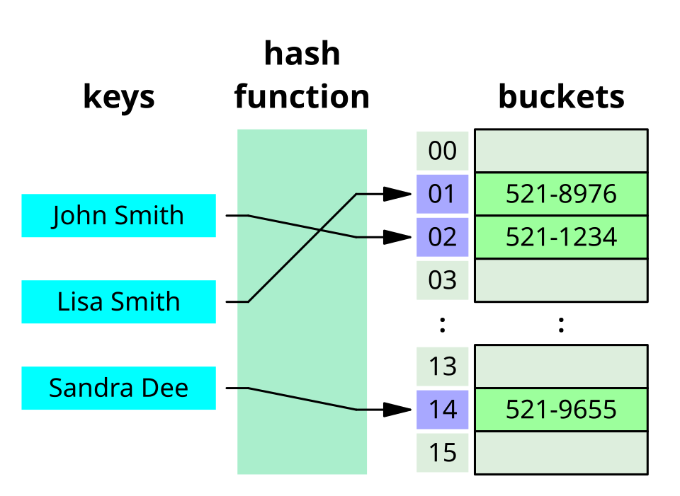
A hash table turns a key into an array index by running it through a hash function, then reads or writes that slot directly. Because indexing an array is O(1), lookup by arbitrary key becomes O(1) too — which is a genuinely surprising result, and the reason dict, HashMap, unordered_map and Object are the most-used structures in programming.

The hash function maps a key directly to a bucket index. No search takes place — the key's own content computes its location. Wikimedia Commons, CC BY-SA 3.0

Core Concepts

Term	Meaning
Hash function	Maps a key to an integer, ideally spreading keys uniformly across the range
Bucket / slot	One entry in the backing array
Collision	Two distinct keys hashing to the same bucket — unavoidable, and the whole design problem
Load factor (α)	entries / buckets. The single number governing performance
Rehashing	Allocating a larger array and reinserting everything, when α grows too large

Architecture / Mechanism

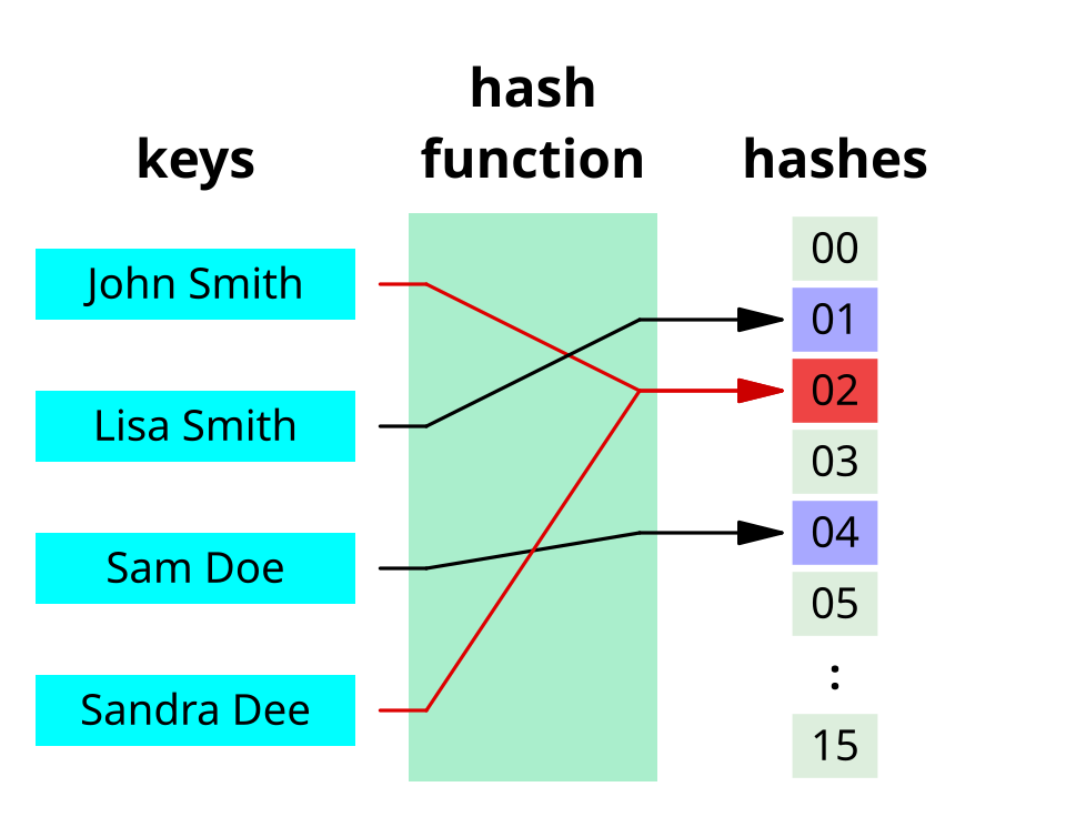
Collisions are not an edge case

With more possible keys than buckets, collisions are guaranteed by pigeonhole. They arrive far earlier than intuition suggests: by the birthday paradox, 23 keys in 365 buckets already collide with probability > 50%.

Two different keys, one bucket. Everything below is about what to do at this moment. Wikimedia Commons, Public domain

The two resolution strategies

Separate chaining — each bucket holds a container (classically a linked list, sometimes a tree) of all entries that landed there:

bucket 01 -> ("Lisa Smith", 521-8976)
bucket 02 -> ("John Smith", 521-1234) -> ("Sandra Dee", 521-9655)
bucket 03 -> (empty)

Open addressing — everything lives in the array itself, and a collision probes for another free slot by a fixed rule (linear probing: try the next slot; quadratic; double hashing):

def insert_linear_probe(table, key, value):
    i = hash(key) % len(table)
    while table[i] is not None and table[i][0] != key:
        i = (i + 1) % len(table)     # walk forward until a free slot
    table[i] = (key, value)

	Separate chaining	Open addressing
Load factor tolerated	> 1 works, degrades gracefully	Must stay below ~0.7, collapses near 1.0
Memory	Pointer per entry, plus nodes	No per-entry overhead, but empty slots
Cache behaviour	Poor — chains chase pointers	Excellent — probes are sequential
Deletion	Simple: unlink	Awkward: needs tombstones
Used by	Java HashMap, older C++ unordered_map	Python dict, Rust HashMap, Go maps, Swift

Most modern implementations chose open addressing, and the reason is the cache column.

Load factor is the dial that controls everything

Linear probing is cheaper than chaining across most of the range — until roughly α = 0.8, where clustering takes over and the cost explodes. Wikimedia Commons, Public domain

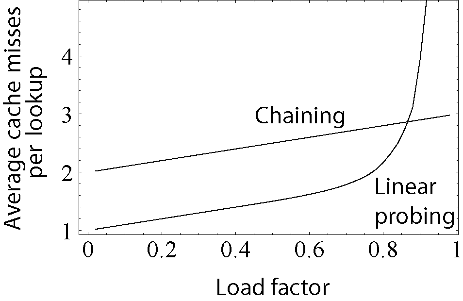
This curve is why implementations rehash. When α crosses a threshold (0.75 in Java, ~0.66 in Python, 0.875 in Rust's hashbrown), the table allocates a larger array — usually double — and reinserts every entry. Rehashing is O(n), but it happens rarely enough to be O(1) amortized, by the same doubling argument as dynamic arrays.

Practical Usage

# Pre-size when the count is known, to avoid repeated rehashing
seen = dict()                      # Python: no capacity argument
# Java:  new HashMap<>(expectedSize / 0.75f + 1)
# C++:   m.reserve(expectedSize)
# Go:    make(map[string]int, expectedSize)

# The classic use: turning a nested scan into a single pass
def two_sum(nums, target):
    seen = {}                      # value -> index
    for i, x in enumerate(nums):
        if target - x in seen:     # O(1) instead of an inner loop
            return seen[target - x], i
        seen[x] = i
    return None

That rewrite — replacing an O(n²) nested scan with an O(n) pass and a hash table — is the single most common application of the structure, and worth recognising on sight.

Edge Cases & Pitfalls

Mutating a key after insertion loses the entry

An entry's bucket is determined by the key's hash at insertion time. Mutate the key and its hash changes, but the entry does not move — so the table now looks in the wrong bucket, and the entry is unreachable while still consuming space.

Python and Rust prevent this structurally by requiring keys to be immutable/hashable. Java does not: a mutable object used as a HashMap key, mutated afterwards, is a silent and genuinely hard-to-find leak. Use immutable keys.

• equals and hashCode must agree. Two keys that compare equal must hash equally, or lookups fail unpredictably. Overriding one without the other is the classic Java bug; the same contract exists as __eq__/__hash__ in Python and Eq/Hash in Rust.
• Worst case is O(n). If every key collides, the table degenerates to a linear scan. Java 8+ converts long chains to red-black trees, capping degradation at O(log n).
• Hash-flooding is a real attack. An attacker who can predict your hash function can force collisions deliberately and turn an O(1) endpoint into O(n) — a denial of service from ordinary traffic. This is why Python, Rust and others use randomly seeded hashing (SipHash) by default. Never use a fast non-cryptographic hash on attacker-controlled keys without a per-process seed.
• Iteration order is not insertion order in general. Python's dict has guaranteed insertion order since 3.7 and Go deliberately randomises it; do not rely on either unless the language promises it.

Comparisons

	Hash table	Balanced BST
Lookup	O(1) expected	O(log n) guaranteed
Worst case	O(n) (O(log n) if treeified)	O(log n)
Ordering	None	Sorted
Range queries, min/max, successor	Not supported	Natural
Memory	Empty slots or chain overhead	Two pointers per node
Choose it when	You look up exact keys	You need order, ranges, or worst-case bounds

References

• Cormen, Leiserson, Rivest & Stein, Introduction to Algorithms, Ch. 11 — hash tables, chaining, open addressing, and universal hashing.
• CPython dict design notes — the compact, insertion-ordered open-addressing design used since 3.6.
• Crosby & Wallach, "Denial of Service via Algorithmic Complexity Attacks" — the paper that made hash-flooding a mainstream concern.

Books & Videos

• Sedgewick & Wayne, Algorithms, 4th ed., §3.4 — hash tables with both collision strategies implemented and measured.

Related Pages

• Arrays & Dynamic Arrays — the backing store, and the source of the amortized-rehash argument.
• Balanced Trees — the ordered alternative.
• Searching Algorithms — where hashing sits among the ways to find things.