Network Flow

A flow network is a directed graph where every edge has a capacity, one vertex is a source pumping flow in, and one is a sink draining it out. The question is how much can flow from source to sink at once, respecting every edge's capacity and requiring that flow into any other vertex equals flow out of it — conservation, the same law that governs water in pipes or current in wires. It sounds like a narrow question about literal networks, but an enormous range of combinatorial problems — matching, scheduling, image segmentation, project selection — turn out to be a max-flow question once the right graph is built, which is why this page spends as much time on modeling as on the algorithm.

The central fact is the max-flow min-cut theorem: the maximum amount of flow that can cross from source to sink exactly equals the minimum total capacity of any "cut" — a partition of the vertices into a source side and a sink side — summed over edges crossing from the source side to the sink side. That the two quantities, one a maximization and the other a minimization, are always equal is proved in CLRS and used here without re-proof; treat it as a fact you can rely on, the way you rely on the triangle inequality.

Core Concepts

Term	Meaning
Flow network	Directed graph, edge capacities, one source s, one sink t
Flow	An assignment of a value to every edge, 0 ≤ flow(u,v) ≤ capacity(u,v), satisfying conservation at every non-s, non-t vertex
Residual capacity	capacity(u,v) − flow(u,v) — how much more can still go forward on this edge, plus a reverse edge of capacity flow(u,v) representing "undo"
Augmenting path	A path from s to t in the residual graph along which every edge has positive residual capacity
Cut	A partition of vertices into S (containing s) and T (containing t); its capacity is the sum of capacities of edges from S to T
Max-flow min-cut theorem	The maximum flow value equals the minimum cut capacity, always (CLRS 4th ed., Thm 24.6)

Mechanism

A max flow (left number on each edge) saturating a minimum cut. No augmenting path exists from source to sink once this flow is reached — every path is blocked by at least one saturated edge. Wikimedia Commons, CC BY-SA 3.0

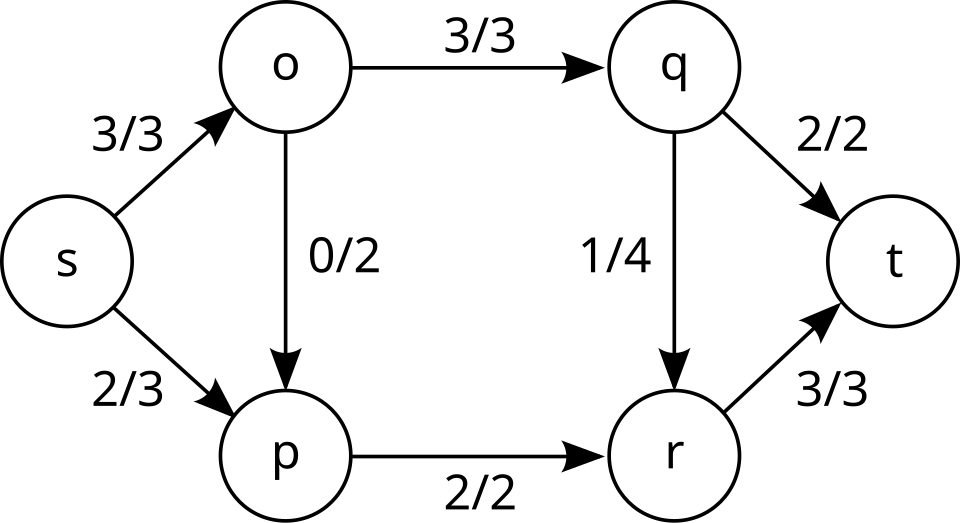
Ford-Fulkerson: augment until stuck

The Ford-Fulkerson method repeats one step: find any path from s to t in the current residual graph, push flow equal to the smallest residual capacity on that path (the bottleneck), update residual capacities forward and backward, and repeat until no path remains. Pushing flow along an edge always creates or enlarges a reverse residual edge — that reverse edge is what lets a later augmentation cancel an earlier, suboptimal choice instead of getting stuck with it permanently.

Trace input — vertices s, a, b, t; capacities s→a 3, s→b 2, a→b 1, a→t 2, b→t 3. Augmenting paths found by BFS (this is Edmonds-Karp — see below), shortest path first:

initial residual capacities (forward only, no flow pushed yet):
  s->a 3   s->b 2   a->b 1   a->t 2   b->t 3

round 1: BFS from s finds s-a-t (2 edges, shortest available)
  bottleneck = min(s->a=3, a->t=2) = 2
  push 2: s->a: 3-2=1 (reverse a->s: 0+2=2)   a->t: 2-2=0 (reverse t->a: 0+2=2)
  flow so far: 2

round 2: BFS from s finds s-b-t (2 edges; s-a-t is now blocked, a->t is 0)
  bottleneck = min(s->b=2, b->t=3) = 2
  push 2: s->b: 2-2=0 (reverse b->s: 0+2=2)   b->t: 3-2=1 (reverse t->b: 0+2=2)
  flow so far: 4

round 3: BFS from s: s->b is now 0, so only s->a (residual 1) is reachable; from a, a->t is
  0 but a->b (residual 1) reaches b, and b->t still has residual 1 -> path s-a-b-t (3 edges)
  bottleneck = min(s->a=1, a->b=1, b->t=1) = 1
  push 1: s->a: 1-1=0   a->b: 1-1=0   b->t: 1-1=0
  flow so far: 5

round 4: BFS from s: s->a is 0, s->b is 0 -> no vertex reachable from s -> no augmenting path
  algorithm terminates. Max flow = 5.

The minimum cut is S = {s, a}, T = {b, t}: the edges crossing it are s→b (2), a→b (1), and a→t (2), summing to exactly 5 — matching the flow found, as the theorem guarantees. Every edge crossing that cut is fully saturated in the final flow, which is always true of a minimum cut: an unsaturated crossing edge would itself be an unused augmenting opportunity.

Python

from collections import deque, defaultdict

def edmonds_karp(capacity, s, t):
    """capacity: {(u, v): cap}. Returns (max_flow, residual capacity dict)."""
    residual = defaultdict(int, capacity)
    graph = defaultdict(set)
    for u, v in capacity:
        graph[u].add(v)
        graph[v].add(u)                          # residual reverse edges may be used too

    def bfs_path():
        parent = {s: None}
        queue = deque([s])
        while queue:
            u = queue.popleft()
            if u == t:
                path = []
                while parent[u] is not None:
                    path.append((parent[u], u))
                    u = parent[u]
                return list(reversed(path))
            for v in graph[u]:
                if v not in parent and residual[(u, v)] > 0:
                    parent[v] = u
                    queue.append(v)
        return None

    max_flow = 0
    while (path := bfs_path()) is not None:
        bottleneck = min(residual[edge] for edge in path)
        for u, v in path:
            residual[(u, v)] -= bottleneck
            residual[(v, u)] += bottleneck
        max_flow += bottleneck
    return max_flow, residual

C++

#include <cassert>
#include <climits>
#include <map>
#include <queue>
#include <set>
#include <string>
#include <vector>

using Capacity = std::map<std::pair<std::string, std::string>, int>;

int edmonds_karp(Capacity residual, const std::string& s, const std::string& t) {
    std::map<std::string, std::set<std::string>> graph;
    for (const auto& [edge, cap] : residual) {
        graph[edge.first].insert(edge.second);
        graph[edge.second].insert(edge.first);
    }

    int max_flow = 0;
    while (true) {
        std::map<std::string, std::string> parent;
        parent[s] = "";
        std::queue<std::string> q;
        q.push(s);
        bool found = false;
        while (!q.empty() && !found) {
            std::string u = q.front(); q.pop();
            for (const auto& v : graph[u]) {
                if (!parent.count(v) && residual[{u, v}] > 0) {
                    parent[v] = u;
                    if (v == t) { found = true; break; }
                    q.push(v);
                }
            }
        }
        if (!found) break;

        std::vector<std::pair<std::string, std::string>> path;
        for (std::string v = t; v != s;) {
            std::string u = parent[v];
            path.push_back({u, v});
            v = u;
        }
        int bottleneck = INT_MAX;
        for (const auto& e : path) bottleneck = std::min(bottleneck, residual[e]);
        for (const auto& [u, v] : path) {
            residual[{u, v}] -= bottleneck;
            residual[{v, u}] += bottleneck;
        }
        max_flow += bottleneck;
    }
    return max_flow;
}

Edmonds-Karp: why BFS gives $O(VE^{2})$

Ford-Fulkerson as stated leaves "find any augmenting path" unspecified — with a careless choice (say, DFS to whichever neighbor comes first) on integer capacities, it still terminates, but the number of augmentations can be proportional to the capacity values themselves, not the graph size: a famous worst case takes as many rounds as the largest capacity, no matter how small the graph. Edmonds-Karp is Ford-Fulkerson with one specific rule — always augment along a shortest path (fewest edges, found by BFS) — and that rule alone bounds the number of augmentations by $O(V \cdot E)$, each BFS costing $O(E)$, for a total of $O(VE^{2})$ (CLRS 4th ed., Thm 24.8). The argument: every augmentation saturates at least one edge on its path (a "critical" edge), and it can be shown that the shortest-path distance from s to any fixed vertex only ever increases across augmentations, never decreases, over the whole run — a monotonicity that limits each edge to being critical at most $O(V)$ times, giving $O(VE)$ total augmentations.

Practical Usage

• scipy.sparse.csgraph.maximum_flow implements a Dinic's-algorithm variant directly on a sparse capacity matrix — see the SciPy documentation for its FlowResult (flow value plus the residual). This is what to reach for before hand-rolling Edmonds-Karp on anything but a teaching example.
• networkx.algorithms.flow.maximum_flow exposes several algorithms including Edmonds-Karp by name (networkx.algorithms.flow.edmonds_karp) — useful when the specific algorithm's behavior, not just the answer, matters for a comparison.
• Bipartite matching as flow. Connect a super-source to every left vertex (capacity 1 each), every original edge (capacity 1), and every right vertex to a super-sink (capacity 1 each). The max flow equals the maximum bipartite matching size, and any integral flow corresponds directly to a matching — this is why bipartite matching admits a flow-based algorithm at all.
• Project selection. Given projects with profits (possibly negative) and prerequisite dependencies, build a source connected to profitable projects, a sink connected from unprofitable ones, infinite capacity along dependency edges, and the min cut identifies exactly which projects to fund for maximum net profit — a classical reduction (CLRS 4th ed., §24.4, "the maximum-flow problem" set of applications; the specific project-selection framing is a common exercise built on the same min-cut argument).

capacity = {
    ("s", "a"): 3, ("s", "b"): 2,
    ("a", "b"): 1, ("a", "t"): 2, ("b", "t"): 3,
}
flow, residual = edmonds_karp(capacity, "s", "t")
assert flow == 5                                        # matches the hand trace above
assert residual[("s", "a")] == 0 and residual[("s", "b")] == 0   # both source edges saturated
# the min cut {s,a} vs {b,t}: crossing capacities 2 + 1 + 2 = 5, matching the flow found
cut_capacity = capacity[("s", "b")] + capacity[("a", "b")] + capacity[("a", "t")]
assert cut_capacity == flow

Edge Cases & Pitfalls

• Anti-parallel edges (u→v and v→u both present with real capacity) break the simple "one residual entry per unordered pair" bookkeeping — split one of the two into a path through a dummy vertex, or track residual capacity per directed edge, not per pair.
• Forgetting the reverse residual edge makes the algorithm correct only when the very first choice of augmenting path happens to be optimal — with it omitted, a suboptimal early augmentation can never be undone, and the algorithm can terminate below the true maximum flow.
• Floating-point capacities. Ford-Fulkerson's convergence proof assumes capacities that decrease by a fixed positive amount each augmentation; irrational or poorly-rounded floating-point capacities can make the classic (non-BFS) version fail to terminate in the worst case. Edmonds-Karp's $O(VE)$ augmentation bound does not depend on capacity values, which is one more reason to prefer it.
• Multiple sources or sinks. Add a single super-source connected to every real source (and a single super-sink from every real sink) with infinite capacity — do not try to run the algorithm with more than one of each directly.
• Confusing flow value with an edge's flow. The value of a flow is the net amount leaving s (or arriving at t) — not the sum of every edge's flow, which double-counts internal edges.

Comparisons

	Time (worst)	Augmenting path rule
Ford-Fulkerson (unspecified path)	$O(E \cdot f*)$, f* the max flow value	Any path — pseudo-polynomial, capacity-dependent
Edmonds-Karp	$O(VE^{2})$	Shortest path by edge count (BFS)
Dinic's algorithm	$O(V^{2}E)$ general, $O(E \cdot sqrt(V))$ on unit-capacity graphs	Blocking flow per phase over a level graph
Push-relabel	$O(V^{2}E)$ to $O(V^{3})$ depending on variant	No augmenting-path search at all — local relabel/push operations

Edmonds-Karp is the right default because its bound holds regardless of the capacities involved. Dinic's algorithm improves on it by finding an entire blocking flow per BFS phase instead of one path at a time, which is why it dominates on the unit-capacity graphs that bipartite matching reduces to.

Recall

InvariantMax-flow min-cut: the maximum flow from source to sink equals the minimum total capacity of any cut separating them — always, and it is used here as a theorem, not re-derived.

Costs

Ford-Fulkerson, any path (worst)$O(E\cdot f\ast )$

Edmonds-Karp, BFS shortest path (worst)$O(V{E}^2)$

Dinic's, unit-capacity graphs (worst)$O(E\cdot sqrt(V))$

single BFS augmentation (worst)$O(E)$

Reach for itA source-to-sink capacity limit to saturate, or a combinatorial problem — matching, selection under dependencies — that can be reframed as one.

TrapOmitting the reverse residual edge when pushing flow. Without it, an early augmenting choice can never be undone, and the algorithm can terminate with less than the true maximum flow.

References

• Cormen, Leiserson, Rivest & Stein, Introduction to Algorithms, 4th ed., Ch. 24 — the max-flow min-cut theorem (Thm 24.6), Ford-Fulkerson, and the Edmonds-Karp analysis (Thm 24.8).
• Sedgewick & Wayne, Algorithms, 4th ed., §6.4 "Maximum Flow" — the same algorithms with a residual-graph-first presentation and worked examples.
• L. R. Ford Jr. & D. R. Fulkerson, "Maximal Flow Through a Network", Canadian J. Mathematics 8, 1956 — the original method.
• J. Edmonds & R. M. Karp, "Theoretical Improvements in Algorithmic Efficiency for Network Flow Problems", J. ACM 19(2), 1972 — the BFS shortest-augmenting-path bound.
• SciPy csgraph.maximum_flow documentation — the library implementation most Python code actually calls.

Related Pages

• Bipartite Graphs & 2-Coloring — maximum matching restated as unit-capacity max flow.
• Traversal: BFS & DFS — the shortest-path search Edmonds-Karp runs on every augmentation.
• Shortest Paths — a different optimization over the same kind of weighted graph.
• Minimum Spanning Trees — another network-design problem, connecting instead of routing flow.