Randomized Algorithms & Sampling

A deterministic algorithm has exactly one worst case, and if that worst case is realistic — an adversary chooses the input, or the input just happens to be sorted, or reverse-sorted, or built from a small alphabet — the worst case is what actually happens. Quicksort picking the first element as its pivot is $O(n \log n)$ on random data and $O(n^{2})$ on already-sorted data, and "already sorted" is not an exotic input; it is a common one. A randomized pivot does not make the $O(n^{2})$ case impossible — some sequence of coin flips could still produce it — it makes that sequence exponentially unlikely for any fixed input, because the bad case now depends on the random choices rather than on what an adversary can arrange in advance.

That reframing — trading a guaranteed bound on one input for a probabilistic bound on every input — is the organizing idea behind this whole page. Las Vegas algorithms always give the correct answer and let randomness affect only the running time (randomized quicksort: always sorts correctly, sometimes slowly). Monte Carlo algorithms fix the running time and let randomness affect correctness (Miller-Rabin primality testing: always finishes in the same bounded time, and returns "probably prime" with a controllable, shrinkable error probability). Both trade a bad worst case for an average case an adversary cannot target — and both depend on the random source actually behaving randomly, which is where the specific algorithms on this page — shuffling and sampling — earn their keep.

Core Concepts

Term	Meaning
Las Vegas algorithm	Always correct; running time is a random variable (e.g. randomized quicksort)
Monte Carlo algorithm	Fixed running time; correctness is probabilistic, with a controllable error rate (e.g. Miller-Rabin)
Fisher-Yates shuffle	Produces a uniformly random permutation in $O(n)$, by picking each element's final position exactly once
Reservoir sampling	Selects k uniform-random items from a stream of unknown length in one pass, $O(n)$ time, $O(k)$ space
Adversarial input	An input specifically constructed to trigger a deterministic algorithm's worst case

Mechanism

Trace input — Fisher-Yates shuffle on [A, B, C, D], walking from the last index down to the first and swapping each position with a uniformly random earlier-or-equal one:

array: [A, B, C, D]   indices 0..3

i = 3: draw j uniformly from [0, 3] -> j = 1        swap(3, 1): [A, D, C, B]
i = 2: draw j uniformly from [0, 2] -> j = 2        swap(2, 2): [A, D, C, B]   (no visible change)
i = 1: draw j uniformly from [0, 1] -> j = 0        swap(1, 0): [D, A, C, B]
i = 0: loop ends (nothing left to swap with)

final shuffled array: [D, A, C, B]

Every one of the 4! = 24 permutations of [A, B, C, D] is reachable by some sequence of draws, and each is reachable by exactly one sequence — which is exactly what "uniformly random permutation" requires: not merely that the output looks mixed, but that no permutation is more likely than any other.

Outcome distribution over many trials, 3-element array: correct Fisher-Yates lands on all 6 permutations with equal frequency; the buggy variant (drawing j from the full range instead of [0, i]) visibly favors some permutations over others. Generated for this page

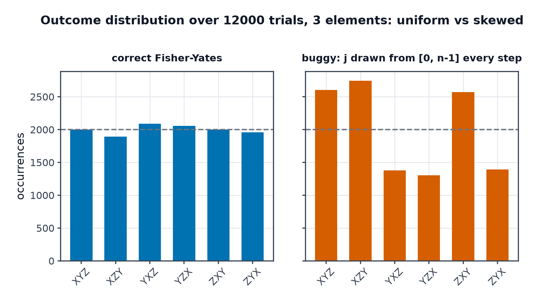
The classic bug is drawing j from the whole array ([0, n-1]) instead of from [0, i] at each step. It still produces "a shuffle" — every element still moves — but the resulting distribution is measurably not uniform: some permutations become more likely than others, because some final positions can be reached by more distinct sequences of draws than others. This is the shuffle equivalent of a hash function that looks random but is not — passing an eyeball test while failing the actual guarantee the algorithm exists to provide.

Python

import random


def fisher_yates(items):
    """Uniformly random permutation in O(n) worst case (Sedgewick & Wayne 4/e, s2.4 exercise)."""
    a = list(items)
    for i in range(len(a) - 1, 0, -1):
        j = random.randint(0, i)          # inclusive of i itself -- the bug is randint(0, n - 1)
        a[i], a[j] = a[j], a[i]
    return a


def fisher_yates_buggy(items):
    """The classic off-by-one: draws j from the WHOLE array every step, not [0, i]."""
    a = list(items)
    n = len(a)
    for i in range(n - 1, 0, -1):
        j = random.randint(0, n - 1)      # bug: should be random.randint(0, i)
        a[i], a[j] = a[j], a[i]
    return a

C++

#include <algorithm>
#include <cassert>
#include <random>
#include <vector>

template <typename T>
void fisher_yates(std::vector<T>& a, std::mt19937& rng) {
    for (std::size_t i = a.size() - 1; i > 0; --i) {
        std::uniform_int_distribution<std::size_t> dist(0, i);     // inclusive of i
        std::swap(a[i], a[dist(rng)]);
    }
}

template <typename T>
void fisher_yates_buggy(std::vector<T>& a, std::mt19937& rng) {
    std::uniform_int_distribution<std::size_t> dist(0, a.size() - 1);   // bug: whole array, every step
    for (std::size_t i = a.size() - 1; i > 0; --i) std::swap(a[i], a[dist(rng)]);
}

Practical Usage

• Python's random.shuffle implements Fisher-Yates correctly and should always be preferred over a hand-written version in real code — the function above exists to show the mechanism and its bug, not to be reused.
• random.sample implements reservoir-style sampling internally for population sizes it cannot fit in memory, and uniform sampling without replacement in general.
• Reservoir sampling answers "pick k random items from a stream whose length is not known in advance" — item i (0-indexed, i >= k) is kept with probability k / (i + 1) when it arrives, replacing a uniformly random existing reservoir slot. The induction (CLRS 4th ed., Problem 5-2): assume every one of the first i items is in the reservoir with probability k / i after processing them. Item i (the (i+1)-th item) is inserted with probability k / (i + 1) by construction — the base case. An item already in the reservoir survives round i either because item i was rejected (probability 1 - k/(i+1)) or because item i was accepted but did not pick that particular slot to evict (probability k/(i+1) * (k-1)/k); summing those two cases and multiplying by the inductive hypothesis k / i simplifies to k / (i + 1) again — so every item seen so far keeps a uniform k / (i + 1) chance of surviving, without ever storing more than k of them.
• Randomized pivots and hashing. Quicksort's randomized-pivot variant turns the $O(n^{2})$ worst case from "any sorted input" into "an exponentially unlikely sequence of draws," and hash tables seed their hash function randomly per process for the same reason — an attacker who can predict a deterministic hash can construct keys that all collide, forcing $O(n)$ operations that should be $O(1)$ expected.

Python

random.seed(0)

# both variants preserve every element (correctness); only the distribution differs
original = ["A", "B", "C", "D"]
result = fisher_yates(original)
assert sorted(result) == sorted(original)
assert len(result) == 4

# the buggy variant is measurably non-uniform: over many trials some permutations
# of a 3-element array occur far more often than 1/6 of the time
from collections import Counter

trials = 6000
correct_counts = Counter(tuple(fisher_yates(["X", "Y", "Z"])) for _ in range(trials))
buggy_counts = Counter(tuple(fisher_yates_buggy(["X", "Y", "Z"])) for _ in range(trials))
assert len(correct_counts) == 6                       # all 6 permutations of 3 items appear
correct_spread = max(correct_counts.values()) - min(correct_counts.values())
buggy_spread = max(buggy_counts.values()) - min(buggy_counts.values())
assert buggy_spread > correct_spread                  # buggy variant is measurably more skewed

C++

int main() {
    std::mt19937 rng(0);
    std::vector<int> a{1, 2, 3, 4};
    auto sorted_before = a;
    fisher_yates(a, rng);
    std::sort(sorted_before.begin(), sorted_before.end());
    auto sorted_after = a;
    std::sort(sorted_after.begin(), sorted_after.end());
    assert(sorted_before == sorted_after);   // same multiset of elements, just reordered
}

Edge Cases & Pitfalls

• The off-by-one shuffle bug. Drawing j from [0, n-1] instead of [0, i] at every step (as in fisher_yates_buggy above) is the single most common shuffle bug — the array still looks mixed, passes casual inspection, and even preserves the same multiset of elements. Only a distribution test (as done in the runnable trace above) reveals it is not uniform.
• Trusting random for security. Python's random module is explicitly documented as not suitable for security or cryptographic purposes — use secrets when unpredictability against an adversary, not just statistical uniformity, is required.
• Confusing "randomized" with "always fast". A randomized pivot makes the $O(n^{2})$ quicksort case exponentially unlikely, not impossible — it is still theoretically possible to draw the exact sequence of pivots that triggers it; the guarantee is about the expected case over the algorithm's own randomness, not a worst-case bound.
• Re-seeding or reusing a fixed seed in production. A fixed random seed makes a randomized algorithm deterministic again, silently reintroducing the exact adversarial-input vulnerability randomization exists to remove — an attacker who learns the seed can construct the same worst case as if the pivot or hash were unrandomized.

Comparisons

	Correctness	Running time	Example
Las Vegas	Always correct	Random variable (expected bound, worst case still possible)	Randomized quicksort
Monte Carlo	Probabilistic, error rate controllable	Fixed	Miller-Rabin primality test
Deterministic	Always correct	Fixed worst case, adversary-targetable	First-element-pivot quicksort

Las Vegas trades a fixed worst-case time for a guarantee of correctness plus a good expected time; Monte Carlo trades a small, controllable chance of being wrong for a hard guarantee on time — the right choice depends on which of the two (a wrong answer, or an unpredictable delay) the calling code can least afford.

Recall

InvariantRandomization does not make a deterministic algorithm's bad case impossible -- it makes the sequence of random choices that triggers it exponentially unlikely for any fixed input, which is what removes an adversary's ability to target it.

Costs

Fisher-Yates shuffle, n elements (worst)$O(n)$

reservoir sampling, k items from a stream of n (worst)$O(n)$

randomized quicksort (expected)$O(n\log n)$

randomized quicksort (worst, exponentially unlikely)$O(n^2)$

Monte Carlo primality test, one round (worst)$O(\log n)$ multiplications

Reach for itA deterministic algorithm whose worst case is a realistic input (sorted data, adversarial keys) rather than an exotic edge case -- randomize the choice the adversary would otherwise control.

TrapThe off-by-one shuffle bug: drawing the swap index from the whole array instead of [0, i] at each step still looks shuffled but is measurably non-uniform.

References

• Cormen, Leiserson, Rivest & Stein, Introduction to Algorithms, 4th ed., §5.3 "Randomized algorithms" and Problem 5-2 — randomized hiring, the shuffle correctness proof, and reservoir sampling's derivation.
• Sedgewick & Wayne, Algorithms, 4th ed., §2.4 exercises — Fisher-Yates as the standard shuffle and its role in randomized quicksort's analysis.
• random — Python docs — shuffle, sample, and the explicit warning against using this module for security purposes; see secrets for the cryptographic alternative.

Related Pages

• Math & Number Theory — the folder's map of where this arithmetic surfaces elsewhere.
• Quicksort — the randomized-pivot variant this page's adversarial-input argument justifies.
• Hash Tables — randomized hash seeding, the same defense against an adversary applied to hashing instead of sorting.
• Combinatorics & Counting — the counting arguments (like the 24 equally likely permutations traced above) that justify a randomized algorithm's guarantees.
• Top-K & Streaming — reservoir sampling in its natural setting.