Searching Algorithms — Overview

Every algorithm in this folder answers the same question — "is this value present, and where" — but each one pays for the answer differently. Linear search pays nothing up front and $O(n)$ every time it runs. Binary search pays $O(n \log n)$ once, up front, to sort the data, and $O(\log n)$ on every lookup after that. A hash table pays $O(n)$ to build and $O(1)$ expected per lookup, at the cost of any ordering.

None of these is "the best search algorithm" in the abstract. The right choice is a question about your workload — how many times you look something up before the data changes underneath you — not a question about which algorithm is cleverest. This page works that trade-off out with actual arithmetic, because "sorting is worth it if you search often enough" is true but useless until you know what "often enough" means for your n.

In This Section

• Linear Search — check each element. No preconditions, no preparation, and the only option when there is no ordering to exploit.
• Binary Search — halve the search space each step. Requires sorted, random-access data, and is notoriously easy to get subtly wrong at the boundaries.
• Binary Search on the Answer — the same halving idea applied to a range of candidate answers instead of an array, for problems phrased as "find the smallest/largest value for which a condition holds."
• Exponential & Ternary Search — exponential search for unbounded or streamed input where the size is not known in advance, and ternary search for finding an extremum of a unimodal function rather than a target value.

The Options, Compared

Approach	Preparation	Per lookup	Requires	Also gives you
Linear search	None	$O(n)$	Nothing	Works on any sequence, any predicate
Binary search	$O(n \log n)$ sort	$O(\log n)$	Sorted, random access	Range queries, nearest match, insertion point
Hash table	$O(n)$ build	$O(1)$ expected	Hashable keys	Nothing else — no ordering
Balanced BST	$O(n \log n)$ build	$O(\log n)$	Comparable keys	Ordering, ranges, and cheap updates

The Cost of the Precondition

Binary search's $O(\log n)$ lookup is not free — it is a rate you buy by paying an $O(n \log n)$ entrance fee to sort first. Whether that trade is worth it depends entirely on $q$, the number of lookups you intend to run before the data changes again.

Compare the two totals directly, for $n$ elements and $q$ queries:

$$\underbrace{q \cdot n}_{\text{repeated linear search}} \quad\text{versus}\quad \underbrace{n \log_2 n + q \log_2 n}_{\text{sort once, then binary search each time}}$$

Sorting wins exactly when the second expression is smaller than the first. Solve for the break-even point $q^{*}$:

$$q \cdot n = n \log_2 n + q \log_2 n \;\;\Longrightarrow\;\; q (n - \log_2 n) = n \log_2 n \;\;\Longrightarrow\;\; q^{*} = \frac{n \log_2 n}{n - \log_2 n}$$

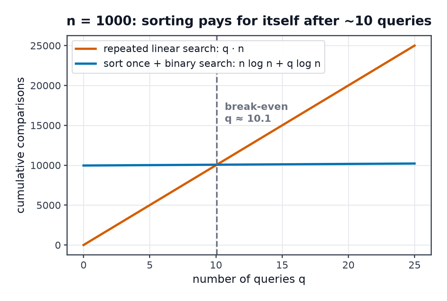
For any $n$ large enough that $\log_2 n \ll n$ (true for essentially every $n$ worth searching), the $-\log_2 n$ term in the denominator barely moves the answer, and $q^{*} \approx \log_2 n$. The break-even point is, to a very good approximation, one query per bit of the data's size — a genuinely small number of queries, which is why binary search's up-front cost so rarely dominates in practice.

n = 1,000: repeated linear search (q·n) grows linearly in q; sort-once-then-binary-search (n log n + q log n) grows far more slowly. The two cross at q ≈ 10.1 — after ten queries, sorting has already paid for itself.

Do not sort inside a loop to enable a binary search

This is a genuinely common performance bug. Sorting costs $O(n \log n)$ and a single binary search saves at most $O(n) - O(\log n)$ over a linear scan, so re-sorting on every lookup is strictly worse than never sorting at all — you pay the full entrance fee every time and use it once. Sort once outside the loop, or reach for a structure that stays sorted incrementally (balanced BST) if the data keeps changing.

Worked Example: n = 1,000

Plugging $n = 1{,}000$ into the exact break-even formula:

log2(1000) ≈ 9.9658

q* = (1000 * 9.9658) / (1000 - 9.9658)
   = 9965.8 / 990.0342
   ≈ 10.066

So for a thousand elements, the eleventh query is where sorting-then-binary-searching becomes cheaper in total than eleven separate linear scans — check the arithmetic directly:

q = 10  linear: 10 * 1000        = 10,000
       sorted: 1000*9.9658 + 10*9.9658 = 9965.8 + 99.658  =  10,065.5   (sorted still costs more)

q = 11  linear: 11 * 1000        = 11,000
       sorted: 1000*9.9658 + 11*9.9658 = 9965.8 + 109.62  =  10,075.4   (sorted now wins)

Ten queries: linear search is still cheaper in total. Eleven queries: sorting has paid for itself. This is also why "sort once, binary search $\log_2 n$ times" is the textbook justification for treating $q \approx \log_2 n$ as the rule of thumb, and why it holds up almost regardless of $n$ — doubling $n$ to two million only moves the break-even point from about 10 to about 21.

Deciding

Recall

InvariantEvery search method trades preparation cost for per-lookup cost; the right choice is set by q, the number of lookups you run before the data changes, not by which algorithm is cleverest.

Costs

linear search, per lookup (worst)$O(n)$

sort once, worst case$O(n\log n)$

binary search, per lookup (worst)$O(\log n)$

break-even query countq* ≈ log2 n

hash table, per lookup (expected)$O(1)$

Reach for itDeciding, before writing any search code, whether the data is queried often enough (roughly log2 n times or more) to justify sorting it first.

TrapRe-sorting inside a loop 'to enable binary search' pays the full $O(n\log n)$ entrance fee on every lookup — strictly worse than never sorting at all.

References

• Knuth, The Art of Computer Programming, Vol. 3, §6.1 (sequential search) and §6.2.1 (binary search) — the two baselines this page compares, with their exact comparison counts.
• Cormen, Leiserson, Rivest & Stein, Introduction to Algorithms, 4th ed., §12.1 — binary search trees as the incrementally-updatable alternative to sort-once-then-binary-search.
• Sedgewick & Wayne, Algorithms, 4th ed., §3.1 "Symbol Tables" — frames search structures by exactly this cost trade-off: preparation cost versus per-query cost versus update cost.

Related Pages

• Hash Tables — the $O(1)$ option, and its conditions.
• Balanced Trees — when the data keeps changing.
• Sorting Algorithms — the preparation step binary search depends on.