Counting Sort, Radix Sort & Bucket Sort

Every comparison sort on this page's siblings is bound below by $Ω(n \log n)$ — a fact proved by a decision tree argument (see Choosing a Sort), not by cleverness anyone has failed to find. That bound only applies to algorithms that decide order by comparing elements. If something is known about the keys beyond "they support <" — that they are integers in a bounded range, or that they distribute roughly uniformly over an interval — sorting can run in linear time, because the decision tree argument no longer applies to it at all.

Counting sort exploits a bounded integer range directly: tally how many elements equal each possible value, then place elements by that tally. Radix sort extends this to numbers too large to tally directly, by running counting sort once per digit instead of once over the whole key. Bucket sort takes a different assumption — not a bounded discrete range, but a roughly uniform distribution over a continuous interval — and turns that assumption into buckets small enough to finish sorting fast.

Prerequisites

Comfortable with arrays and with why comparison sorts are bounded below by $Ω(n \log n)$ — see Choosing a Sort for that argument. This page assumes it rather than re-deriving it.

Core Concepts

Term	Meaning
Key range	Counting sort's requirement: keys are integers in [0, k) for some known k
Stable	Equal keys keep their relative input order in the output. A requirement for LSD radix, not a nicety — see Mechanism
LSD radix sort	Sorts by digit starting from the least significant, one stable counting-sort pass per digit
MSD radix sort	Sorts by digit starting from the most significant, recursing into each digit bucket independently
Bucket sort	Distributes elements into b intervals by value, sorts each bucket (usually with insertion sort), concatenates
Radix (base) r	The number of buckets used per digit — 10 for decimal digits, 256 for a byte, any power of two for bit-shift extraction

Mechanism

Counting sort

Given keys in [0, k), counting sort builds a histogram of length k, turns it into a prefix sum (so count[v] becomes "how many elements are ≤ v"), then places each element directly at its final index by reading the input backwards and decrementing the count it consumes. Reading backwards is what makes it stable: two equal keys are placed in reverse order of discovery, which reverse of backwards traversal restores to input order.

Python

def counting_sort(a, k):
    """Stable sort of integers in [0, k). O(n + k) time and space."""
    count = [0] * k
    for v in a:
        count[v] += 1
    for v in range(1, k):
        count[v] += count[v - 1]              # count[v] is now "how many elements are <= v"
    out = [0] * len(a)
    for v in reversed(a):                      # backwards traversal is what makes this stable
        count[v] -= 1
        out[count[v]] = v
    return out

C++

#include <algorithm>
#include <cassert>
#include <vector>

std::vector<int> counting_sort(const std::vector<int>& a, int k) {
    std::vector<int> count(k, 0);
    for (int v : a) ++count[v];
    for (int v = 1; v < k; ++v) count[v] += count[v - 1];
    std::vector<int> out(a.size());
    for (auto it = a.rbegin(); it != a.rend(); ++it) {
        out[--count[*it]] = *it;
    }
    return out;
}

Counting sort's cost is $O(n + k)$, not $O(n \log n)$ — no comparisons happen at all. That is only a win when k = O(n); sorting 32-bit integers directly with k = 2^32 allocates 4 billion counters to sort a handful of values.

LSD radix sort

Radix sort's trick for keys too large to tally in one pass is to tally one digit at a time, from least significant to most, using counting sort as the stable subroutine for each digit. Stability is not incidental here — it is the entire correctness argument. After sorting by digit d, the elements are correctly ordered on digits 0..d, provided ties on digit d preserve whatever order digits 0..d-1 had already established. An unstable per-digit pass would scramble that lower-order information on every tie, and the final result would not be sorted at all.

LSD radix sort of [170, 45, 75, 90, 802, 24, 2, 66]: each pass is one stable counting sort keyed on a single decimal digit, least significant first. The array is fully sorted after the hundreds-digit pass, because no number here has a thousands digit.

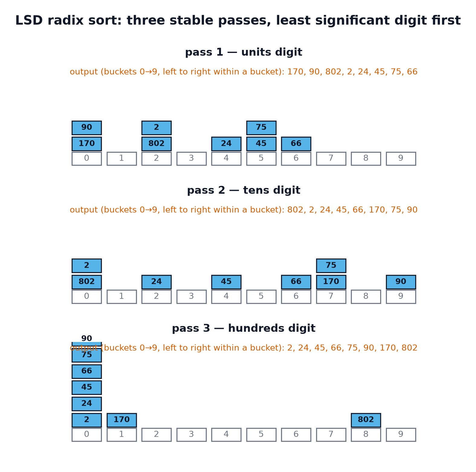
input = [170, 45, 75, 90, 802, 24, 2, 66]

pass 1 (units digit), buckets 0-9, stable within each:
  0: 170, 90     2: 802, 2      4: 24      5: 45, 75      6: 66
  output -> [170, 90, 802, 2, 24, 45, 75, 66]

pass 2 (tens digit), buckets over the pass-1 output:
  0: 802, 2      2: 24      4: 45      6: 66      7: 170, 75      9: 90
  output -> [802, 2, 24, 45, 66, 170, 75, 90]

pass 3 (hundreds digit), buckets over the pass-2 output:
  0: 2, 24, 45, 66, 75, 90       1: 170       8: 802
  output -> [2, 24, 45, 66, 75, 90, 170, 802]   -- fully sorted

Python

def lsd_radix_sort(a, base=10):
    """Sorts non-negative integers by repeated stable counting sort on each digit."""
    if not a:
        return []
    max_val = max(a)
    exp = 1
    out = list(a)
    while max_val // exp > 0:
        count = [0] * base
        for v in out:
            count[(v // exp) % base] += 1
        for d in range(1, base):
            count[d] += count[d - 1]
        placed = [0] * len(out)
        for v in reversed(out):
            d = (v // exp) % base
            count[d] -= 1
            placed[count[d]] = v
        out = placed                           # this pass's output feeds the next digit
        exp *= base
    return out

C++

std::vector<int> lsd_radix_sort(std::vector<int> a, int base = 10) {
    if (a.empty()) return a;
    int max_val = *std::max_element(a.begin(), a.end());
    for (long long exp = 1; max_val / exp > 0; exp *= base) {
        std::vector<int> count(base, 0);
        for (int v : a) ++count[(v / exp) % base];
        for (int d = 1; d < base; ++d) count[d] += count[d - 1];
        std::vector<int> placed(a.size());
        for (auto it = a.rbegin(); it != a.rend(); ++it) {
            int d = (*it / exp) % base;
            placed[--count[d]] = *it;
        }
        a = std::move(placed);
    }
    return a;
}

For n keys of d digits each in base r, LSD radix sort runs d counting-sort passes at $O(n + r)$ each: $O(d(n + r))$ worst case. Treating d and r as constants (fixed-width integers, base 256) gives $O(n)$ — the reason a bounded-key-domain sort can beat the comparison-sort floor.

Python

# both implementations, checked on the traced input
assert counting_sort([4, 2, 2, 8, 3, 3, 1], 9) == [1, 2, 2, 3, 3, 4, 8]
assert lsd_radix_sort([170, 45, 75, 90, 802, 24, 2, 66]) == [2, 24, 45, 66, 75, 90, 170, 802]
assert lsd_radix_sort([]) == []

C++

int main() {
    assert((counting_sort({4, 2, 2, 8, 3, 3, 1}, 9) == std::vector<int>{1, 2, 2, 3, 3, 4, 8}));
    assert((lsd_radix_sort({170, 45, 75, 90, 802, 24, 2, 66})
            == std::vector<int>{2, 24, 45, 66, 75, 90, 170, 802}));
}

MSD radix sort and bucket sort

MSD radix sort processes the most significant digit first and recurses into each of that digit's buckets independently, the same shape as quicksort's partition-then-recurse. This makes it usable on variable-length keys such as strings — an MSD pass past a string's last character defines it as smaller than any string it shares a prefix with, and the recursion naturally stops on single-element or empty buckets. Sedgewick & Wayne 4th ed. §5.1 covers this string-sorting form (American flag sort / MSD string sort) in detail and gives it $O(n)$ average time for keys with independent random characters — worse in the worst case, since a group of keys sharing a long common prefix recurses to the prefix's full depth before any digit distinguishes them.

Bucket sort makes a different assumption: keys are real numbers roughly uniformly distributed over a known interval, say [0, 1). It allocates n buckets, drops each key v into bucket ⌊v · n⌋, sorts each bucket with insertion sort (buckets are expected to be tiny), and concatenates. Under the uniformity assumption each bucket holds $O(1)$ elements in expectation, so total work is $O(n)$ expected, not worst case — CLRS 4th ed. §8.4 proves this via linearity of expectation over the bucket sizes. A skewed distribution (all keys near 0.999) defeats the assumption and degrades to one bucket holding everything, at which point bucket sort is just insertion sort on the whole array: $O(n^{2})$ worst case.

Practical Usage

• Python has no built-in counting or radix sort. sorted() is Timsort, a comparison sort — see Choosing a Sort. Reach for counting sort by hand only when the key range is known and small, e.g. sorting bytes, small integer scores, or histogram bucketing.
• numpy.argsort(kind="stable") (NumPy docs) uses radix sort internally for integer and unsigned-integer dtypes when it is faster than the default quicksort — an implementation detail exposed only through the kind parameter's documented stability guarantee, not through a name you ask for directly.
• Database engines and external sorts use radix/bucket-style partitioning to split a dataset into disjoint, independently sortable ranges before an external merge — see External & Parallel Sorting for the disk-bound version of the same idea.
• Suffix array construction (not covered on this page) uses LSD-radix-style sorting on (rank, rank) pairs as its inner step, because a bounded integer range is exactly what rank pairs are.

Edge Cases & Pitfalls

• Forgetting to read backwards in counting sort. Reading forwards while decrementing counts still produces a sorted array, but it silently reverses the relative order of equal keys — the sort becomes unstable without any visible symptom until something downstream (a radix pass, or a caller relying on the guarantee) breaks.
• Using an unstable sort as radix sort's per-digit pass. This is not a performance bug, it is a correctness bug: the result is not sorted. Any per-digit routine that reorders ties is disqualified, no matter how fast.
• Choosing k too large for counting sort. k sets both the time and the space; counting sort on 32-bit keys with k = 2^32 is a memory-allocation failure waiting to happen, not a fast sort.
• Negative numbers. Both counting sort and the radix sort above assume non-negative keys. A bias offset (v - min(a)) or a separate sign pass is required before the loop above applies — omitting it makes (v // exp) % base behave inconsistently across languages, since Python's // floors toward negative infinity while C++'s integer division truncates toward zero.
• Bucket sort on a skewed distribution. The $O(n)$ expected bound assumes uniformity; a real dataset that is skewed (timestamps clustered at the top of the hour, prices clustered at round numbers) can collapse most elements into one bucket and degrade toward $O(n^{2})$.

Comparisons

	Best	Average	Worst	Space	Stable	In-place
Counting sort	$O(n + k)$	$O(n + k)$	$O(n + k)$	$O(n + k)$	Yes	No
LSD radix sort	$O(d(n + r))$	$O(d(n + r))$	$O(d(n + r))$	$O(n + r)$	Yes	No
MSD radix sort	$O(n)$	$O(n)$ average (independent random keys, Sedgewick & Wayne 4th ed. §5.1)	$O(n \cdot d)$	$O(n + r)$	Yes (stable variant)	No
Bucket sort	$O(n)$	$O(n)$ expected (CLRS 4th ed. §8.4, uniform keys)	$O(n^{2})$	$O(n)$	Depends on the per-bucket sort	No
Mergesort (for reference)	$O(n \log n)$	$O(n \log n)$	$O(n \log n)$	$O(n)$	Yes	No

Every row above beats mergesort's $O(n \log n)$ worst case in its favourable regime, and every row's win comes from an assumption the comparison-sort proof doesn't get to make: a bounded range, a fixed digit count, or a known distribution. Violate the assumption and the row's bound stops holding — bucket sort in particular is the only one of the four whose worst case is quadratic, because unlike counting or radix sort it has no way to force the assumption to hold.

Recall

InvariantCounting sort, radix sort, and bucket sort are not faster comparison sorts — they sidestep the $\Omega (n\log n)$ comparison-sort bound entirely by using something known about the keys (a bounded range, a fixed digit width, a distribution) instead of comparing them.

Costs

counting sort (worst)$O(n+k)$

LSD radix sort, d digits, base r (worst)$O(d(n+r))$

MSD radix sort, independent random keys (average)$O(n)$

bucket sort, uniform keys (expected)$O(n)$

bucket sort, skewed keys (worst)$O(n^2)$

Reach for itKeys that are integers in a known bounded range, fixed-width (IDs, bytes, small scores), or floats known to be roughly uniform over an interval — never a first choice for arbitrary comparable keys.

TrapUsing an unstable sort as LSD radix sort's per-digit subroutine. It is not a slowdown, it is a correctness bug: ties on a low-order digit get scrambled and the array comes out unsorted.

References

• Cormen, Leiserson, Rivest & Stein, Introduction to Algorithms, 4th ed., §8.2 (counting sort), §8.3 (radix sort), §8.4 (bucket sort) — the linear-time sorts, their invariants, and the proof that bucket sort's $O(n)$ bound is an expectation over a uniformity assumption.
• Sedgewick & Wayne, Algorithms, 4th ed., §5.1 "String Sorts" — LSD and MSD string sort (key-indexed counting applied per character), including three-way radix quicksort as a hybrid.
• NumPy argsort documentation — the kind="stable" guarantee and where NumPy actually uses radix sort internally.

Related Pages

• Choosing a Sort — the $Ω(n \log n)$ comparison-sort lower bound these three algorithms sidestep, and why a bounded-key assumption is what makes that legal.
• Mergesort — the comparison-sort baseline every row in the table above is measured against.
• Quicksort — MSD radix sort's partition-then-recurse shape, with a digit test in place of a comparison.
• Arrays — the contiguous buffers these algorithms read and write in place of the input.