Insertion Sort

Insertion sort builds the sorted result one element at a time, taking the next element and sliding it back into its correct place among those already sorted — exactly how most people sort a hand of playing cards.

It is $O(n^2)$, and it is nonetheless the most used of the elementary sorts, because it is inside almost every production sorting routine. Below roughly 16–32 elements it beats quicksort and mergesort outright, so those algorithms hand their small subarrays to it.

The prefix on the left is always sorted. Each new element shifts left past everything larger than it, then drops into place. Wikimedia Commons, CC BY-SA 3.0

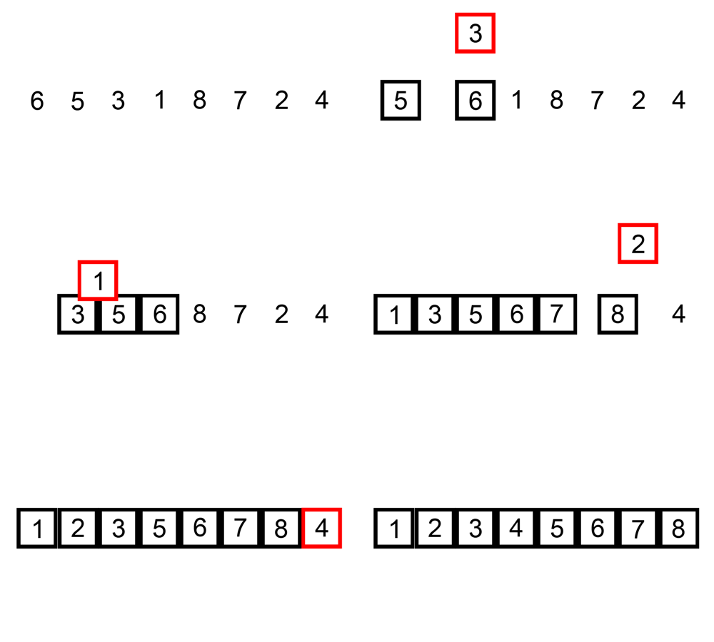
Core Concepts

Property	Value
Best case	$O(n)$ — already sorted; one comparison per element, no shifts
Average	$O(n^2)$
Worst case	$O(n^2)$ — reverse sorted
Space	$O(1)$
Stable	Yes
Adaptive	Yes, strongly — $O(n + d)$ where d is the number of inversions
Online	Yes — can sort a stream as elements arrive

Mechanism

Python

def insertion_sort(a):
    for i in range(1, len(a)):
        key = a[i]
        j = i - 1
        # Shift everything greater than key one position right
        while j >= 0 and a[j] > key:
            a[j + 1] = a[j]
            j -= 1
        a[j + 1] = key      # drop key into the gap
    return a

C++

#include <cassert>
#include <cstddef>
#include <vector>

void insertion_sort(std::vector<int>& a) {
    for (std::size_t i = 1; i < a.size(); ++i) {
        int key = a[i];
        int j = static_cast<int>(i) - 1;
        // Shift everything greater than key one position right
        while (j >= 0 && a[j] > key) {
            a[j + 1] = a[j];
            --j;
        }
        a[j + 1] = key;     // drop key into the gap
    }
}

Note that the inner loop shifts rather than swaps — one write per displaced element instead of three. That is roughly a 3× constant-factor win over the swap-based formulation, and it is why insertion sort outperforms bubble sort on the same asymptotics.

Tracing [5, 1, 8, 3]:

Step	Key	Action	Result
i=1	1	shift 5 right, insert 1 at index 0	[1, 5, 8, 3]
i=2	8	8 > 5, no shift needed, insert 8 at index 2	[1, 5, 8, 3]
i=3	3	shift 8 right, shift 5 right, insert 3 at index 1	[1, 3, 5, 8]

Why "adaptive" is the important word

The inner loop runs only while elements are out of order, so the total work is proportional to the number of inversions — pairs that are in the wrong relative order. Formally the cost is $O(n + d)$, and for nearly-sorted data d is small:

Input	Inversions	Cost
Already sorted	0	$O(n)$
One element out of place	$O(n)$	$O(n)$
Every element within k positions of its home	$O(nk)$	$O(nk)$
Reverse sorted	n(n−1)/2	$O(n^2)$

Real data is very often nearly sorted — appended log lines, mostly-ordered records, a sorted list with a few recent additions. This property is what Timsort is built to exploit.

Practical Usage

Python

# doc:no-run
# Illustrative fragment: partition() and insertion_sort_range() are not defined here.
# The way insertion sort is actually used: as the base case of a bigger sort
SMALL = 16

def hybrid_sort(a, lo, hi):
    if hi - lo < SMALL:
        insertion_sort_range(a, lo, hi)     # cheap, cache-friendly, no recursion
        return
    p = partition(a, lo, hi)
    hybrid_sort(a, lo, p)
    hybrid_sort(a, p + 1, hi)

C++

// doc:no-run
// Illustrative fragment: partition() and insertion_sort_range() are not defined here.
// The way insertion sort is actually used: as the base case of a bigger sort
constexpr int SMALL = 16;

void hybrid_sort(std::vector<int>& a, int lo, int hi) {
    if (hi - lo < SMALL) {
        insertion_sort_range(a, lo, hi);        // cheap, cache-friendly, no recursion
        return;
    }
    int p = partition(a, lo, hi);
    hybrid_sort(a, lo, p);
    hybrid_sort(a, p + 1, hi);
}

The reason this wins below the threshold: insertion sort has almost no per-element overhead, does no recursion, allocates nothing, and touches memory strictly sequentially. Quicksort's partitioning and recursion cost more than the quadratic term saves at those sizes.

Binary insertion sort — using binary search to find the insertion point — reduces comparisons to $O(n \log n)$ but leaves the shifting at $O(n^2)$. It helps only when comparisons are much more expensive than moves.

Why it is the cutoff inside introsort and Timsort

Two real standard-library sorts fall back to insertion sort below a size threshold, for the same underlying reason: at small n, insertion sort's low constant factor beats the recursive structure of a faster asymptotic algorithm outright, and both libraries measured that trade rather than assumed it.

• Introsort — C++'s std::sort. libstdc++'s implementation partitions with quicksort down to ranges of 16 elements (the constant _S_threshold in its <bits/stl_algo.h>), then finishes the entire array with one pass of insertion sort at the end rather than recursing into every small range individually — insertion sort on an almost-sorted array (each element already within 16 positions of home) costs $O(nk)$ for small k, which is cheaper than n/16 separate small sorts once data movement is fully accounted for. The C++ standard requires std::sort's complexity to be $O(n \log n)$ comparisons ([alg.sort]); the specific 16-element cutoff and the insertion-sort finish are libstdc++'s implementation choice for meeting that requirement, not something the standard mandates directly.
• Timsort — Python's sorted() and list.sort(). Timsort's MIN_RUN is chosen (typically 32–64, picked so that n / MIN_RUN is close to a power of two) so that every detected run is extended up to at least that length using binary insertion sort before merging begins — using binary search to find each element's insertion point keeps the comparison count at $O(n \log n)$ even though the shifting is still $O(n^2)$ in the worst case, which is fine precisely because runs are kept short. This is documented directly in CPython's own design notes (listsort.txt), which states the binary-insertion-sort extension explicitly as the mechanism for turning short runs into merge-ready ones.

Both designs are making the identical bet insertion sort's adaptivity analysis predicts: below some small, empirically-chosen n, or on any range that is already nearly sorted, insertion sort's $O(n + d)$ behavior beats a fast sort's constant overhead and recursion cost.

Python

# checked on the traced input
assert insertion_sort([5, 1, 8, 3]) == [1, 3, 5, 8]
assert insertion_sort([1, 2, 3]) == [1, 2, 3]     # zero shifts needed
assert insertion_sort([]) == []

C++

int main() {
    std::vector<int> a{5, 1, 8, 3};
    insertion_sort(a);
    assert((a == std::vector<int>{1, 3, 5, 8}));
}

Edge Cases & Pitfalls

• Swapping instead of shifting triples the writes for no benefit. Write the shift form.
• The j >= 0 bound must come first in the while condition; reversing the operands indexes a[-1] in Python (silently wrapping to the end) rather than failing.
• Use > not >= in the comparison. >= shifts past equal elements and destroys stability.
• It is still $O(n^2)$. The adaptivity is real, but on genuinely random input of any size it loses badly — this is a small-input and nearly-sorted-input tool.

Comparisons

	Insertion	Bubble	Selection
Best case	$O(n)$	$O(n)$	$O(n^2)$
Writes on random input	~$n^2$/4 shifts	~$n^2$/2 swaps (×3 writes)	n − 1 swaps
Stable	Yes	Yes	No
Adaptive	Strongly	Weakly	No
Online	Yes	No	No
Used in practice	Yes — inside Timsort, introsort, pdqsort	No	Rarely

Recall

InvariantThe inner loop shifts only while an element is out of order, so total work is proportional to n plus the number of inversions — d — rather than always n^2.

Costs

best case (already sorted)$O(n)$

average case$O(n^2)$

worst case (reverse sorted)$O(n^2)$

adaptive cost, d inversions$O(n+d)$

extra space$O(1)$

Reach for itSmall n (below ~16-32 elements) or data that is already nearly sorted — which is also exactly why faster sorts call this one as their base case instead of recursing all the way down.

TrapUsing >= instead of > in the shift comparison. It still produces a sorted array, but shifts past equal elements and silently destroys stability.

References

• Cormen, Leiserson, Rivest & Stein, Introduction to Algorithms, 4th ed., §2.1 — insertion sort is the book's first algorithm, with its loop invariant proved in full.
• Sedgewick & Wayne, Algorithms, 4th ed., §2.1 — the inversion-count analysis behind the adaptivity claim.
• C++ standard, [alg.sort] — std::sort's required complexity ($O(n \log n)$ comparisons); the small-range insertion-sort cutoff is an implementation choice for meeting that requirement, not part of the standard's text.
• CPython listsort.txt — Timsort's own design notes, including the binary-insertion-sort extension of short runs up to MIN_RUN.

Books & Videos

• VisuAlgo — Sorting — run it against nearly-sorted input to see the adaptivity directly.

Related Pages

• Choosing a Sort — Timsort and introsort, where this algorithm actually lives.
• Quicksort — the sort that delegates its small subarrays here.