Mergesort

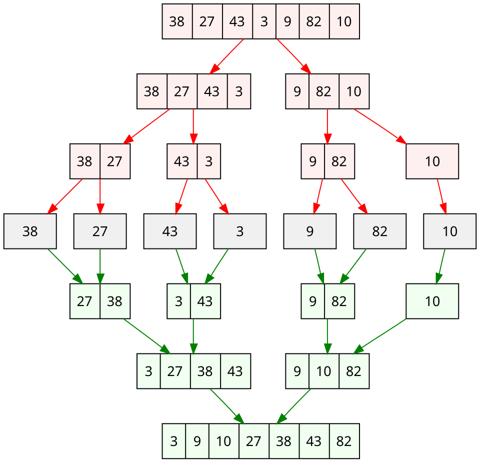
Mergesort splits the array in half, sorts each half recursively, and merges the two sorted halves back together. The insight is that merging two already-sorted sequences is linear — you compare their two front elements and take the smaller, repeatedly.

Splitting costs nothing and produces log n levels; merging costs $O(n)$ per level. Hence $O(n \log n)$, on every input, with no worst case to worry about.

Splitting down (red) does no comparisons at all. All the work is in merging back up (green), where each level touches every element exactly once. Wikimedia Commons, Public domain

Core Concepts

Property	Value
Best case	$O(n \log n)$
Average	$O(n \log n)$
Worst case	$O(n \log n)$ — guaranteed
Space	$O(n)$ — the merge buffer
Stable	Yes
Adaptive	No, in the classic form (but see Timsort)
Parallelises	Well — the two halves are independent

Mechanism

Python

def merge_sort(a):
    if len(a) <= 1:
        return a
    mid = len(a) // 2
    left = merge_sort(a[:mid])          # sort each half
    right = merge_sort(a[mid:])
    return merge(left, right)

def merge(left, right):
    out, i, j = [], 0, 0
    while i < len(left) and j < len(right):
        if left[i] <= right[j]:         # <= keeps the sort stable
            out.append(left[i]); i += 1
        else:
            out.append(right[j]); j += 1
    out.extend(left[i:])                # one side is exhausted; append the rest
    out.extend(right[j:])
    return out

C++

#include <algorithm>
#include <cassert>
#include <vector>

std::vector<int> merge(const std::vector<int>& left, const std::vector<int>& right) {
    std::vector<int> out;
    out.reserve(left.size() + right.size());
    auto i = left.begin(), j = right.begin();
    while (i != left.end() && j != right.end())
        out.push_back(*i <= *j ? *i++ : *j++);      // <= keeps the sort stable
    out.insert(out.end(), i, left.end());           // one side is exhausted; append the rest
    out.insert(out.end(), j, right.end());
    return out;
}

std::vector<int> merge_sort(const std::vector<int>& a) {
    if (a.size() <= 1) return a;
    auto mid = a.begin() + static_cast<std::ptrdiff_t>(a.size() / 2);
    auto left  = merge_sort(std::vector<int>(a.begin(), mid));   // sort each half
    auto right = merge_sort(std::vector<int>(mid, a.end()));
    return merge(left, right);
}

Runs double in length at each level: 1, 2, 4, 8… The array is sorted after log₂ n merge passes. Wikimedia Commons, CC BY-SA 3.0

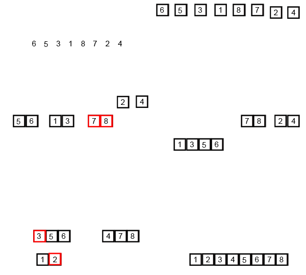
Tracing the single merge step on left = [1, 5] and right = [3, 8], element by element:

Step	i, j	Compare	Take	Output so far
1	i=0, j=0	left[0]=1 vs right[0]=3	1 (left)	[1]
2	i=1, j=0	left[1]=5 vs right[0]=3	3 (right)	[1, 3]
3	i=1, j=1	left[1]=5 vs right[1]=8	5 (left)	[1, 3, 5]
4	i=2, j=1	left exhausted	append remaining right ([8])	[1, 3, 5, 8]

Four elements, at most four comparisons (three real comparisons, then one exhaustion check) — a merge of two runs of total length n never does more than n − 1 comparisons, which is the entire basis for the $O(n)$-per-level claim below.

Why the complexity is exactly $O(n \log n)$

The recursion halves the input, so it has $\log_2 n$ levels. Every level merges a total of n elements, regardless of how they are distributed across subarrays. Work per level is therefore $Θ(n)$, and the total is $Θ(n \log n)$ — with no dependence on the data, which is why best, average and worst are all the same.

Stability comes from one character

left[i] <= right[j] takes from the left run when elements compare equal. Since the left run holds elements that came earlier in the original array, equal elements keep their original order. Change it to < and the merge takes from the right on ties, silently destroying stability.

Practical Usage

Mergesort is the right choice when:

• Stability is required — sorting by a secondary key after a primary one.
• Worst-case guarantees matter — real-time or adversarial contexts where quicksort's $O(n^2)$ is unacceptable.
• The data does not fit in memory. External mergesort reads sorted runs from disk and merges them with sequential I/O, which is the one access pattern storage is good at. This is how databases sort tables larger than RAM.
• You are sorting a linked list. Merging lists needs only pointer rewiring — $O(1)$ extra space, no random access required. This is the one case where mergesort is better on a list than on an array.
• You want to parallelise. The two recursive calls share nothing.

Python

# Bottom-up mergesort — no recursion, same complexity
def merge_sort_iterative(a):
    width = 1
    while width < len(a):
        for i in range(0, len(a), 2 * width):
            a[i:i + 2 * width] = merge(a[i:i + width], a[i + width:i + 2 * width])
        width *= 2
    return a

C++

// Bottom-up mergesort — no recursion, same complexity
void merge_sort_iterative(std::vector<int>& a) {
    auto n = static_cast<std::ptrdiff_t>(a.size());
    for (std::ptrdiff_t width = 1; width < n; width *= 2) {
        for (std::ptrdiff_t i = 0; i < n; i += 2 * width) {
            auto mid = std::min(i + width, n);
            auto end = std::min(i + 2 * width, n);
            std::inplace_merge(a.begin() + i, a.begin() + mid, a.begin() + end);
        }
    }
}

Python

# checked on the traced merge and on the full sort
assert merge([1, 5], [3, 8]) == [1, 3, 5, 8]
assert merge_sort([5, 1, 8, 3]) == [1, 3, 5, 8]
assert merge_sort([]) == []

C++

int main() {
    assert((merge({1, 5}, {3, 8}) == std::vector<int>{1, 3, 5, 8}));
    assert((merge_sort({5, 1, 8, 3}) == std::vector<int>{1, 3, 5, 8}));
}

Edge Cases & Pitfalls

The $O(n)$ space is the real cost

Mergesort cannot merge in place efficiently. Naive in-place merge algorithms exist but are either $O(n^2)$ or have constant factors bad enough to erase the benefit. For a large array this means a second buffer the same size — which can be the deciding factor on memory-constrained systems, and is the main reason quicksort is preferred for in-memory array sorting.

A good implementation allocates one scratch buffer up front and reuses it, rather than allocating per merge as the readable version above does.

• Slicing allocates. The Python above creates new lists at every level — clear, but it does roughly $O(n \log n)$ allocation. Production code passes indices into a single shared buffer.
• < instead of <= in the merge silently loses stability.
• Recursion depth is $O(\log n)$, which is safe — unlike quicksort's worst case.

Comparisons

	Mergesort	Quicksort	Heapsort
Worst case	$O(n \log n)$	$O(n^2)$	$O(n \log n)$
Space	$O(n)$	$O(\log n)$	$O(1)$
Stable	Yes	No	No
Locality	Good — sequential merges	Excellent	Poor — jumps around
Typical speed on arrays	Good	Fastest	Slowest of the three
Linked lists	Ideal	Awkward	Impractical

Recall

InvariantMerging two already-sorted runs is linear — compare the two fronts and take the smaller, repeatedly — so splitting for free plus log n levels of $O(n)$ merging gives $O(n\log n)$ on every input, with no case distinction to make.

Costs

merge of two runs, total length n (worst)$O(n)$

best/average/worst, full sort$O(n\log n)$

extra space (worst)$O(n)$

recursion depth$O(\log n)$

Reach for itStability is required, a worst-case guarantee is required, the data does not fit in memory (external sort), or the input is a linked list where merging costs no extra space at all.

TrapWriting the merge's tie-break as < instead of <=. The output is still sorted, but ties now take from the right run first, silently destroying stability.

References

• Cormen, Leiserson, Rivest & Stein, Introduction to Algorithms, 4th ed., §2.3 — mergesort, and the recurrence-tree analysis of its complexity.
• Knuth, The Art of Computer Programming, Vol. 3, §5.2.4 — merging and external sorting, including multiway merges.

Books & Videos

• VisuAlgo — Sorting — watch the merge levels build up.

Related Pages

• Quicksort — the in-place alternative with a worse worst case.
• Divide & Conquer — the general pattern this instantiates.
• Choosing a Sort — Timsort, which is an adaptive mergesort.