Anomaly Detection

Fraud, equipment failure, network intrusions — the interesting class is often so rare that a supervised classifier never sees enough positive examples to learn from. Anomaly detection reframes the problem entirely: instead of learning what the rare class looks like, learn what normal looks like, and flag anything that deviates.

Key idea

Anomaly detection is what you do when the positive class is too rare, too varied, or too unknown to learn a classifier for.

Anomaly detection models what normal looks like and flags whatever falls far outside it. The contour you pick as the boundary sets the false-positive rate — and that is a business decision, not a statistical one.

Outlier vs. novelty vs. anomaly

Outlier: a point unusual relative to the rest of a static dataset. Novelty: a point unusual relative to a training distribution, encountered at inference time on new data. Anomaly: often used interchangeably with both, sometimes reserved for cases implying an underlying fault or malicious cause. The distinction matters for which sklearn API you use (fit_predict for outlier detection on a fixed set, fit then predict for novelty detection on new points).

When to treat it as classification instead

If you have enough labelled examples of the rare class (even a few hundred) and its patterns are consistent, Imbalanced Data's classification techniques (class weighting, resampling, threshold tuning) often outperform pure anomaly detection — anomaly detection is the fallback for when labels are too scarce or the "abnormal" category is too heterogeneous to model directly.

Statistical methods

• Z-score: flag points more than $k$ standard deviations from the mean — simple, assumes roughly Gaussian data, sensitive to the very outliers it's trying to detect (they inflate the mean and standard deviation used to compute the score).
• IQR (interquartile range): flag points outside $[Q_1 - 1.5\,\text{IQR}, Q_3 + 1.5\,\text{IQR}]$ — more robust than z-score since quartiles are less sensitive to extreme values.
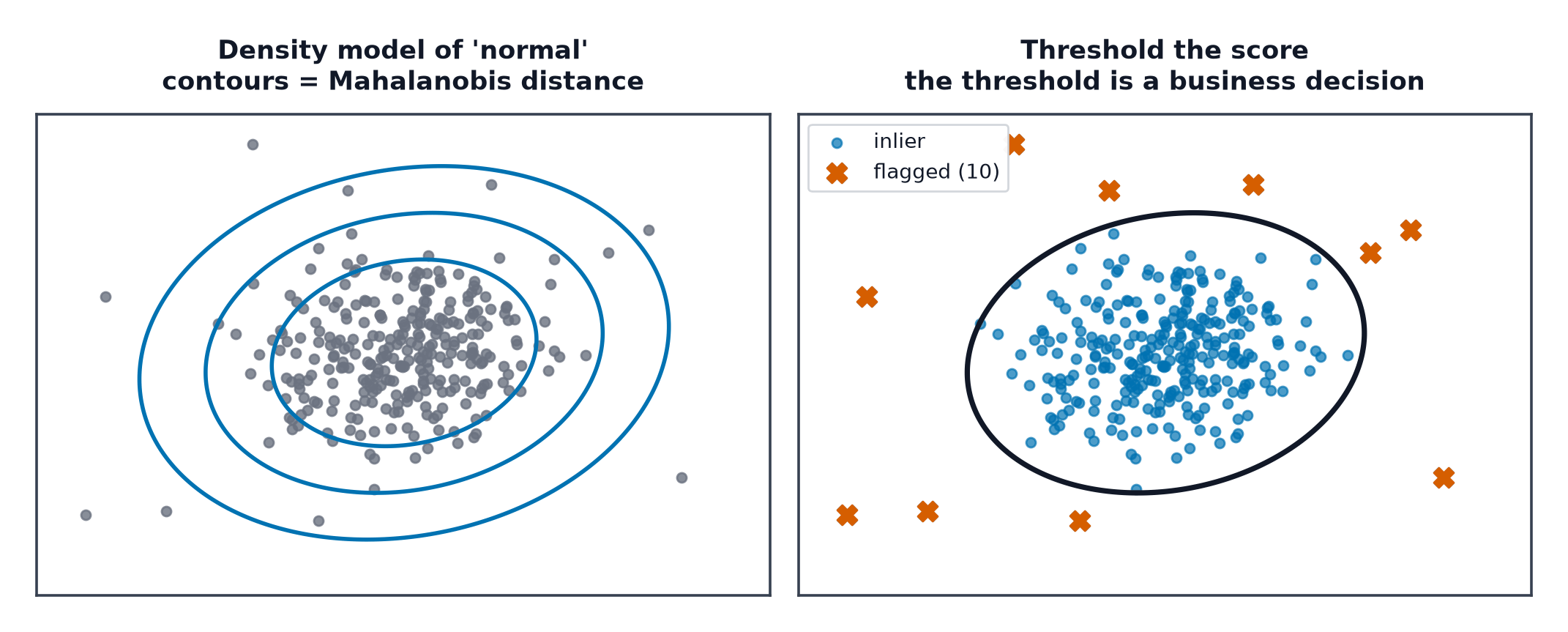
• Mahalanobis distance: generalises z-score to multiple correlated dimensions, accounting for the covariance structure:

$$D_M(x) = \sqrt{(x-\mu)^\top \Sigma^{-1} (x-\mu)}$$

Symbol	Meaning
$\mu, \Sigma$	mean and covariance of the "normal" data
$D_M(x)$	Mahalanobis distance of point $x$ from that distribution

Density methods

KDE (kernel density estimation) and GMM likelihood thresholding (Gaussian Mixture Models) both fit a density estimate to normal data, then flag points with low likelihood under that fitted density — a direct, probabilistic notion of "unusual."

Distance methods

kNN distance: the distance from a point to its $k$-th nearest neighbour — large distance implies an isolated (anomalous) point. LOF (Local Outlier Factor): compares a point's local density to its neighbours' local densities, so it can detect anomalies even in regions where the overall data density varies — a point that's normal-density-for-a-sparse-region but flagged by a single global threshold would be missed by simpler methods.

Isolation Forest

Random splits isolate anomalies faster than normal points, by construction: an anomaly, being rare and different, tends to be separable from the rest of the data in very few random splits, while a normal point buried in a dense cluster requires many splits to isolate. Isolation Forest exploits this directly — it builds random trees and scores each point by the average path length needed to isolate it, with short paths indicating anomalies.

One-class SVM

Learns a boundary enclosing the "normal" region of feature space (using the Kernel Methods trick for non-linear boundaries), and flags points falling outside it — conceptually Support Vector Machines's margin idea applied to a single class instead of separating two.

Autoencoder reconstruction error

Mentioned here, detailed in Autoencoders: train a network to reconstruct normal data; anomalies, being unlike anything the network learned to compress, reconstruct poorly — high reconstruction error becomes the anomaly score.

Evaluation without labels, and with a few labels

Without any labels, evaluation is largely qualitative (do the flagged points look genuinely unusual on manual review?). With even a small labelled sample: precision@k (of the top-$k$ flagged points, how many are true anomalies) and PR-AUC (Evaluation Metrics for Classification) both apply directly, since anomaly detection is fundamentally an extreme case of imbalanced binary classification.

Threshold selection as a business decision

Every method above produces a continuous anomaly score, not a binary label — the cutoff for "flag this" is a decision about the cost of false positives (investigating a normal case) versus false negatives (missing a real anomaly), identical in spirit to the threshold discussion in Evaluation Metrics for Classification.

Code: three methods compared, PR-AUC on labelled imbalanced data

anomaly_detection_demo.py

import numpy as np
import matplotlib.pyplot as plt
from sklearn.ensemble import IsolationForest
from sklearn.neighbors import LocalOutlierFactor
from sklearn.svm import OneClassSVM
from sklearn.metrics import average_precision_score

rng = np.random.default_rng(0)
X_normal = rng.normal(size=(300, 2))
X_anomalies = rng.uniform(-6, 6, size=(15, 2))
X = np.vstack([X_normal, X_anomalies])
y_true = np.array([0] * 300 + [1] * 15)  # 1 = anomaly, held out for evaluation only

models = {
    "Isolation Forest": IsolationForest(contamination=0.05, random_state=0),
    "LOF": LocalOutlierFactor(novelty=False, contamination=0.05),
    "One-Class SVM": OneClassSVM(nu=0.05, kernel="rbf", gamma="auto"),
}

fig, axes = plt.subplots(1, 3, figsize=(15, 4))
xx, yy = np.meshgrid(np.linspace(-6, 6, 200), np.linspace(-6, 6, 200))
for ax, (name, model) in zip(axes, models.items()):
    preds = model.fit_predict(X)  # -1 = anomaly, 1 = normal
    scores = -model.score_samples(X) if hasattr(model, "score_samples") else -model.negative_outlier_factor_
    ap = average_precision_score(y_true, scores)
    ax.scatter(X[:, 0], X[:, 1], c=(preds == -1), cmap="coolwarm", s=15)
    ax.set_title(f"{name}\nPR-AUC={ap:.3f}")
plt.savefig("anomaly_methods_comparison.png")

When to reach for this

Data size	moderate to large for density/distance methods; Isolation Forest scales well
Feature count	low-to-moderate; density estimation suffers the curse of dimensionality
Interpretability	statistical/distance methods: high; Isolation Forest/one-class SVM: lower
Training cost	Isolation Forest: fast; LOF/kNN-distance: $O(n^2)$ without indexing
Inference cost	varies; Isolation Forest and one-class SVM support fast scoring of new points

See also

• Hierarchical and Density-Based Clustering — DBSCAN's noise label as a related anomaly signal.
• Imbalanced Data — the classification-based alternative when some labels are available.