Decision Trees

Every other model in this section requires some statistical literacy to interpret. A decision tree doesn't — you can hand the diagram to someone with no ML background and they can trace a prediction themselves, one yes/no question at a time. That transparency comes at a real cost: trees are greedy, and greedy is not the same as optimal.

Key idea

A tree recursively splits the feature space on whichever single question most reduces impurity — greedy, interpretable, and prone to memorising everything.

Every tree boundary is a union of axis-aligned rectangles — a diagonal separation always costs a staircase of splits. Depth is the capacity knob: at 12 the tree is fencing off individual noise points.

The recursive splitting algorithm

At each node, consider every possible (feature, threshold) split; pick the one that most reduces impurity in the resulting two child nodes; recurse on each child until a stopping condition is met.

Impurity measures: Gini and entropy

$$\text{Gini}(p) = 1 - \sum_k p_k^2, \qquad \text{Entropy}(p) = -\sum_k p_k \log_2 p_k$$

Both measure how mixed the classes are in a node — zero when a node is pure (one class only), maximal when classes are evenly mixed. In practice they produce very similar trees; Gini is slightly cheaper to compute (no logarithm) and is the more common default.

Information gain

$$\text{Gain} = \text{Impurity}(\text{parent}) - \sum_{\text{child}} \frac{n_{\text{child}}}{n_{\text{parent}}} \, \text{Impurity}(\text{child})$$

The split chosen at each node is the one maximising this gain.

Regression trees and variance reduction

For continuous targets, impurity is replaced by variance — a split is chosen to minimise the weighted variance of the target within each resulting child, exactly analogous to Gini/entropy for classification.

Symbol	Meaning
$p_k$	proportion of class $k$ in a node
$n_{\text{child}}, n_{\text{parent}}$	example counts in child/parent nodes

Greedy splitting is not globally optimal

At each step the tree picks the locally best split without considering how it constrains future splits — finding the globally optimal tree is NP-hard, so every practical implementation is this greedy approximation, which can miss combinations of splits that would jointly be better than the sum of their individually-best parts.

Stopping criteria and pruning

Pre-pruning (stop growing early): max depth, minimum samples per leaf, minimum impurity decrease. Post-pruning (grow fully, then trim back): grow an unconstrained tree, then remove branches that don't improve validation performance — generally produces better trees than pre-pruning alone, at higher training cost.

Handling categorical features and missing values

Trees naturally handle categorical splits (partition categories into two groups) and some implementations handle missing values directly by learning a default direction at each split — advantages relative to distance-based or linear methods, which require explicit encoding and imputation first.

Why single trees overfit

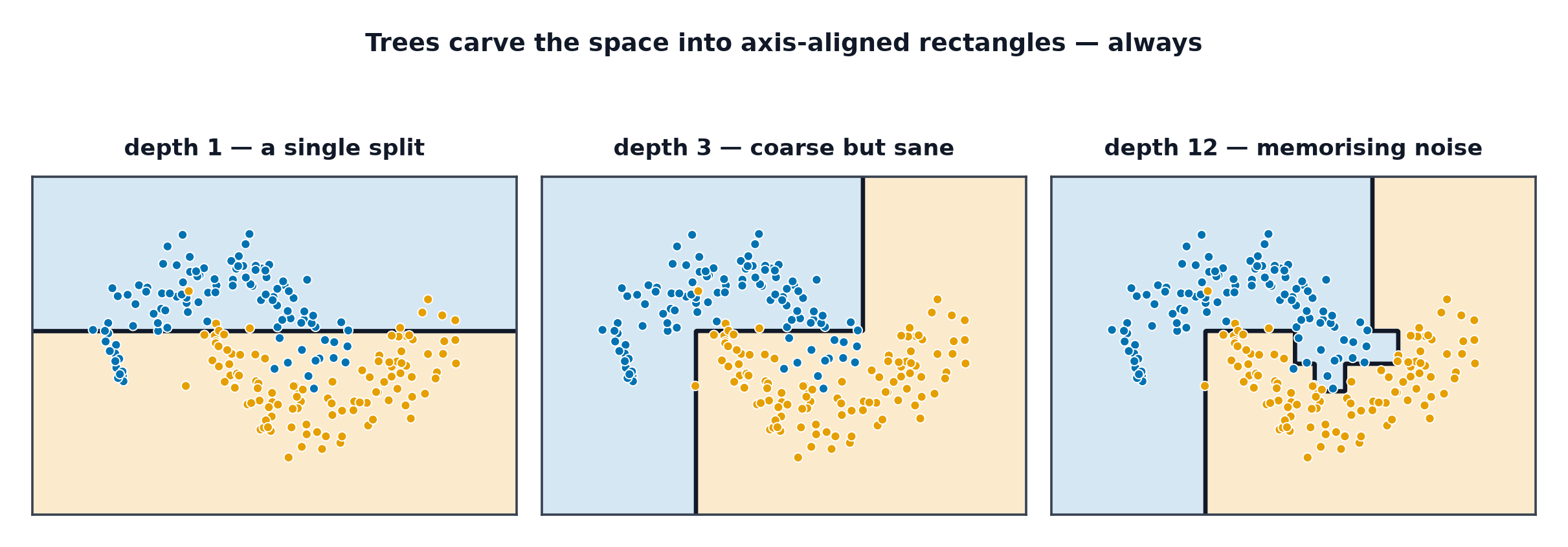
An unconstrained tree can keep splitting until every leaf contains a single training example — perfect training accuracy, achieved by memorising noise, and typically poor generalisation. This is the canonical high-variance model from Bias-Variance Tradeoff.

Feature importance, and its bias

Impurity-based feature importance sums the impurity decrease attributed to each feature across all its splits — but this measure is systematically biased toward high-cardinality features (a feature with many possible split points has more opportunities to appear to reduce impurity, even if it's actually uninformative). Permutation importance (Random Forests and Bagging) avoids this bias.

Axis-aligned boundaries as the core limitation

Every split is a threshold on a single feature, so the decision boundary is always a staircase of axis-aligned segments — a diagonal true boundary requires many small steps to approximate, which trees can do but inefficiently, often needing far more splits (and more data) than a model that can represent diagonals directly.

Code: a tree from scratch, sklearn comparison, the overfitting depth sweep

decision_tree_demo.py

import numpy as np
from sklearn.tree import DecisionTreeClassifier, export_text
from sklearn.datasets import make_classification
from sklearn.model_selection import train_test_split

def gini(y):
    if len(y) == 0: return 0
    p = np.bincount(y) / len(y)
    return 1 - np.sum(p ** 2)

def best_split(X, y):
    best_gain, best_feat, best_thresh = -1, None, None
    parent_impurity = gini(y)
    for feat in range(X.shape[1]):
        for thresh in np.unique(X[:, feat]):
            left_mask = X[:, feat] <= thresh
            if left_mask.sum() == 0 or (~left_mask).sum() == 0:
                continue
            left_imp, right_imp = gini(y[left_mask]), gini(y[~left_mask])
            weighted = (left_mask.sum() * left_imp + (~left_mask).sum() * right_imp) / len(y)
            gain = parent_impurity - weighted
            if gain > best_gain:
                best_gain, best_feat, best_thresh = gain, feat, thresh
    return best_feat, best_thresh, best_gain

X, y = make_classification(n_samples=50, n_features=3, n_informative=2, random_state=0)
feat, thresh, gain = best_split(X, y)
print(f"best root split: feature {feat}, threshold {thresh:.3f}, gain {gain:.3f}")

# --- sklearn tree, printed ---
X_train, X_test, y_train, y_test = train_test_split(X, y, test_size=0.3, random_state=0)
tree = DecisionTreeClassifier(max_depth=3, random_state=0).fit(X_train, y_train)
print(export_text(tree, feature_names=[f"x{i}" for i in range(X.shape[1])]))

# --- Depth sweep: train accuracy hits 1.0, test accuracy degrades ---
print("\ndepth | train acc | test acc")
for depth in [1, 2, 3, 5, 10, None]:
    t = DecisionTreeClassifier(max_depth=depth, random_state=0).fit(X_train, y_train)
    print(f"{str(depth):5s} | {t.score(X_train, y_train):.3f}     | {t.score(X_test, y_test):.3f}")

Unbounded depth should reach or approach 1.0 training accuracy while test accuracy plateaus or degrades — the depth sweep is the bias-variance tradeoff made visible on a single hyperparameter, exactly as with kNN's $k$.

When to reach for this

Data size	any
Feature count	any, mixed numeric/categorical without preprocessing
Interpretability	highest of any non-linear model
Training cost	moderate, roughly $O(n \log n \cdot d)$
Inference cost	very low — a single root-to-leaf path

See also

• Random Forests and Bagging — averaging many trees to fix the overfitting problem.
• Bias-Variance Tradeoff — the theory behind why unconstrained trees overfit.