Gaussian Mixture Models

k-means forces every point into exactly one cluster, with no notion of confidence. A Gaussian mixture model asks a softer question: what's the probability this point belongs to each cluster? Answering it requires an algorithm — expectation-maximisation — that recurs throughout probabilistic ML wherever there are hidden variables to infer.

Key idea

Model the data as a weighted sum of Gaussians and each point gets a probability of belonging to each cluster instead of a hard label.

A GMM generalises k-means in two ways: components can be elliptical rather than spherical, and membership is a probability rather than a hard label. The colour gradient in the right panel is that soft assignment.

The mixture model

$$p(x) = \sum_{k=1}^K \pi_k \, \mathcal{N}(x \mid \mu_k, \Sigma_k)$$

The data is assumed generated by first picking a component $k$ with probability $\pi_k$, then drawing $x$ from that component's Gaussian.

Soft vs. hard assignment

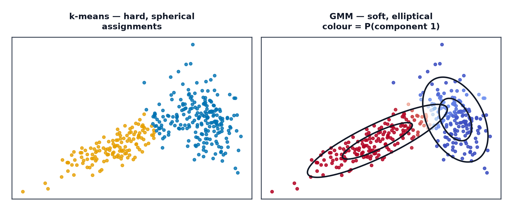
k-means assigns each point to exactly one cluster (hard). A GMM instead computes a full probability distribution over which component generated each point (soft) — a point near the boundary between two clusters gets a genuinely mixed assignment (e.g. 60%/40%) rather than being forced into one or the other.

The EM algorithm

E-step (Expectation): given the current parameters, compute the responsibility $\gamma_{ik}$ — the posterior probability that point $i$ came from component $k$:

$$\gamma_{ik} = \frac{\pi_k \, \mathcal{N}(x_i \mid \mu_k, \Sigma_k)}{\sum_j \pi_j \, \mathcal{N}(x_i \mid \mu_j, \Sigma_j)}$$

M-step (Maximisation): given the responsibilities, update each component's parameters to maximise the (weighted) likelihood:

$$\mu_k = \frac{\sum_i \gamma_{ik} x_i}{\sum_i \gamma_{ik}}, \qquad \pi_k = \frac{1}{n}\sum_i \gamma_{ik}$$

Repeat E and M steps until convergence — this is a chicken-and-egg loop: knowing the responsibilities would make estimating the Gaussians trivial, and knowing the Gaussians would make computing responsibilities trivial, so EM alternates between the two.

Symbol	Meaning
$\pi_k$	mixture weight — prior probability of component $k$
$\gamma_{ik}$	responsibility — posterior probability point $i$ came from component $k$
$\mu_k, \Sigma_k$	mean and covariance of component $k$

Why EM increases likelihood monotonically

Each E-step computes an exact lower bound on the log-likelihood that touches it at the current parameters; each M-step maximises that bound. Since the bound never exceeds the true likelihood but touches it at the start of each iteration, improving the bound can only improve (or leave unchanged) the true likelihood — a guarantee that training never gets worse, though (like k-means) it can still converge to a local optimum.

Covariance types

• Full: each component gets its own arbitrary covariance matrix — most flexible, most parameters.
• Tied: all components share one covariance matrix — fewer parameters, assumes clusters have the same shape.
• Diagonal: covariance matrix constrained to diagonal — assumes features are uncorrelated within a cluster.
• Spherical: a single variance per component, isotropic — the GMM equivalent of k-means' round-cluster assumption.

k-means as a special case of GMM

A GMM with spherical, equal-variance, equal-weight components, in the limit as variance shrinks to zero, produces exactly hard assignments identical to k-means — k-means is a simplified, hard-assignment special case of the more general GMM framework.

Choosing components with BIC/AIC

Unlike k-means' elbow/silhouette heuristics, GMM has a natural model-selection criterion: since it's a genuine probabilistic model, information criteria like BIC (Bayesian Information Criterion) directly penalise both poor fit and excess parameters, giving a principled way to compare different component counts.

Degenerate solutions

A component can collapse onto a single point (variance shrinking toward zero, likelihood diverging to infinity) — a known pathology of unconstrained covariance estimation with too little data per component. Regularisation (a minimum variance floor) or constrained covariance types (tied, diagonal) prevent this.

GMM as a density estimator, not just a clusterer

Beyond assigning points to clusters, a fitted GMM is a complete model of $p(x)$ — usable for anomaly detection (low-likelihood points, see Anomaly Detection), data generation (sample from the fitted mixture), or as a component within a larger probabilistic pipeline.

Code: GMM on elongated clusters, confidence ellipses, BIC curve

gmm_demo.py

import numpy as np
import matplotlib.pyplot as plt
from matplotlib.patches import Ellipse
from sklearn.mixture import GaussianMixture
from sklearn.datasets import make_blobs

rng = np.random.default_rng(0)
X, _ = make_blobs(n_samples=300, centers=2, random_state=0)
X = np.dot(X, [[2, 1], [0, 1]])  # stretch into elongated clusters where k-means struggles

gmm = GaussianMixture(n_components=2, covariance_type="full", random_state=0).fit(X)
labels = gmm.predict(X)

fig, ax = plt.subplots()
ax.scatter(X[:, 0], X[:, 1], c=labels, s=15)
for mean, cov in zip(gmm.means_, gmm.covariances_):
    eigvals, eigvecs = np.linalg.eigh(cov)
    angle = np.degrees(np.arctan2(*eigvecs[:, -1][::-1]))
    width, height = 2 * np.sqrt(eigvals) * 2  # 2-sigma ellipse
    ax.add_patch(Ellipse(mean, width, height, angle=angle, fill=False, edgecolor="red"))
plt.savefig("gmm_ellipses.png")

# --- BIC curve for choosing component count ---
bics = []
for k in range(1, 7):
    m = GaussianMixture(n_components=k, random_state=0).fit(X)
    bics.append(m.bic(X))
print("BIC per component count (1-6):", np.round(bics, 1), "\n  <- should be lowest near k=2, the true count")

# --- Simple E-step / M-step mechanics, shown directly ---
print("\nresponsibilities for first 3 points (soft assignment):")
print(np.round(gmm.predict_proba(X[:3]), 3))

When to reach for this

Data size	small to moderate
Feature count	low-to-moderate; covariance estimation gets expensive in high dimensions
Interpretability	moderate (means, covariances, mixture weights are all inspectable)
Training cost	iterative, similar order to k-means per iteration but more per-iteration work
Inference cost	evaluate the mixture density — cheap

See also

• k-Means Clustering — the hard-assignment special case this generalises.
• Statistics and Estimation — the maximum likelihood framework EM operates within.