Gradient Boosting

Random forests average many independent trees to cancel out variance. Gradient boosting does something structurally different: it builds trees one at a time, each new tree specifically targeting the mistakes the ensemble has made so far. Where bagging reduces variance, boosting reduces bias — and the combination of the two ideas covers most of what wins tabular ML competitions.

Key idea

Fit each new tree to the residual errors of the ensemble so far — boosting reduces bias where bagging reduced variance.

Each stump is fitted to what the ensemble still gets wrong. Individually they are useless; summed with a small learning rate they converge on the target — which is why boosting reduces bias where bagging reduces variance.

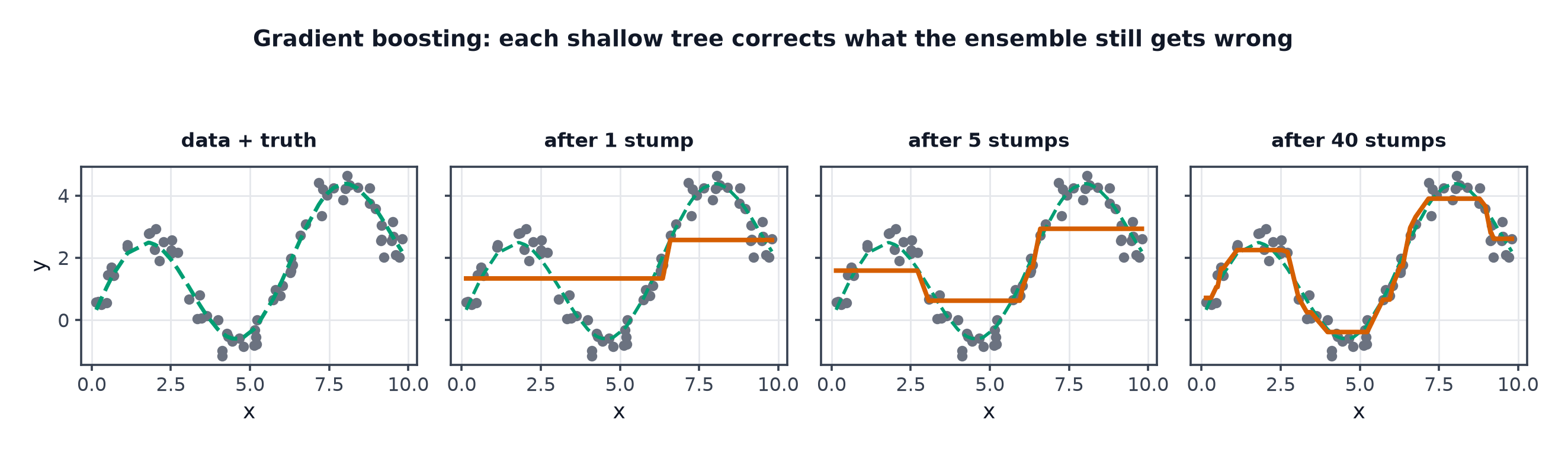
Boosting vs. bagging, side by side

	Bagging	Boosting
Trees built	independently, in parallel	sequentially, each depending on the last
What it reduces	variance	bias
Base learner	typically deep, low-bias trees	typically shallow, high-bias "stumps"
Failure mode	can still be biased if trees are weak	can overfit if run too long

AdaBoost as the historical entry point

AdaBoost reweights misclassified examples after each round, forcing the next weak learner to focus on what the ensemble currently gets wrong — the historical predecessor to gradient boosting, and a useful mental model even though modern implementations use the gradient-based formulation below.

Gradient boosting as gradient descent in function space

Instead of adjusting parameters of a single model, gradient boosting adjusts the function itself, one additive term at a time:

$$F_m(x) = F_{m-1}(x) + \nu \, h_m(x)$$

Each new weak learner $h_m$ is trained to approximate the negative gradient of the loss with respect to the current ensemble's predictions — literally gradient descent, except the "step" is an entire tree rather than a parameter update.

Fitting to pseudo-residuals

For squared-error loss, the negative gradient with respect to the current predictions is exactly the residual $y_i - F_{m-1}(x_i)$ — so each new tree literally fits the errors the ensemble has made so far:

$$r_i = -\left.\frac{\partial L(y_i, F(x_i))}{\partial F(x_i)}\right|_{F=F_{m-1}}$$

Symbol	Meaning
$F_m$	the ensemble's prediction function after $m$ rounds
$h_m$	the weak learner (tree) added at round $m$
$\nu$	learning rate, shrinking each tree's contribution
$r_i$	pseudo-residual — the target the new tree is fit to

The learning rate / n_estimators trade

Small $\nu$ (e.g. 0.01–0.1) requires more trees to reach the same fit but generalises better — this mirrors Learning Rate Schedules's core trade, except here the "steps" are entire trees rather than gradient updates.

Tree depth as interaction order

A depth-1 tree ("stump") can only model a single feature's effect in isolation; depth-2 trees can capture two-way interactions; depth-$k$ trees capture up to $k$-way feature interactions. Boosting typically uses shallow trees (depth 3–6) — deep trees are unnecessary because boosting's sequential structure builds up complexity across many rounds instead of within a single tree.

Subsampling (stochastic gradient boosting)

Training each tree on a random subset of rows (and/or columns) adds randomness that reduces overfitting and speeds up training, borrowing bagging's variance-reduction trick on top of boosting's bias-reduction mechanism.

Regularisation in boosting

Shrinkage ($\nu$), tree depth limits, minimum samples per leaf, and subsampling all act as regularisers — boosting has more knobs than bagging precisely because, unlike bagging, it can overfit by simply running for too many rounds.

Why boosting overfits differently from bagging

Bagging's variance-reduction effect means adding more trees essentially never hurts (it may plateau, but shouldn't get worse). Boosting's bias-reduction mechanism means adding more rounds keeps chasing residuals — eventually including noise — so validation performance can degrade past some optimal number of rounds, unlike bagging.

Early stopping on a validation set

Because more rounds can eventually overfit, track validation loss during training and stop once it stops improving — the same early-stopping principle from Overfitting and Regularization, applied to boosting rounds instead of gradient descent epochs.

Code: depth-2 stumps from scratch, fit improving per round

gradient_boosting_demo.py

import numpy as np
import matplotlib.pyplot as plt
from sklearn.tree import DecisionTreeRegressor
from sklearn.ensemble import GradientBoostingRegressor

rng = np.random.default_rng(0)
X = np.sort(rng.uniform(-3, 3, size=(200, 1)), axis=0)
y = np.sin(X).ravel() + rng.normal(scale=0.2, size=200)

def gradient_boost_fit(X, y, n_rounds, lr=0.1, max_depth=2):
    F = np.zeros(len(y))  # start at F_0 = 0
    trees = []
    for _ in range(n_rounds):
        residuals = y - F  # pseudo-residuals for squared error
        tree = DecisionTreeRegressor(max_depth=max_depth).fit(X, residuals)
        F += lr * tree.predict(X)
        trees.append(tree)
    return trees, F

fig, axes = plt.subplots(1, 3, figsize=(15, 4))
for ax, n_rounds in zip(axes, [1, 10, 100]):
    trees, F = gradient_boost_fit(X, y, n_rounds)
    ax.scatter(X, y, s=10, alpha=0.4)
    ax.plot(X, F, "r-", linewidth=2)
    ax.set_title(f"{n_rounds} rounds")
plt.savefig("boosting_rounds.png")

# --- sklearn, for comparison ---
sk_model = GradientBoostingRegressor(n_estimators=100, learning_rate=0.1, max_depth=2).fit(X, y)
print("sklearn train MSE:", np.mean((sk_model.predict(X) - y) ** 2))

At 1 round the fit is a flat approximation; by 100 rounds it should closely trace the underlying sine wave — direct visual evidence of gradient boosting incrementally reducing bias round by round.

When to reach for this

Data size	small to large
Feature count	handles many features, including mixed types
Interpretability	low without extra tooling (SHAP, permutation importance)
Training cost	higher than random forests — sequential, cannot parallelise across rounds
Inference cost	proportional to number of rounds

See also

• Boosting Libraries: XGBoost, LightGBM, CatBoost — the production-grade implementations of this algorithm.
• Random Forests and Bagging — the variance-reduction counterpart to this bias-reduction method.