Hierarchical and Density-Based Clustering

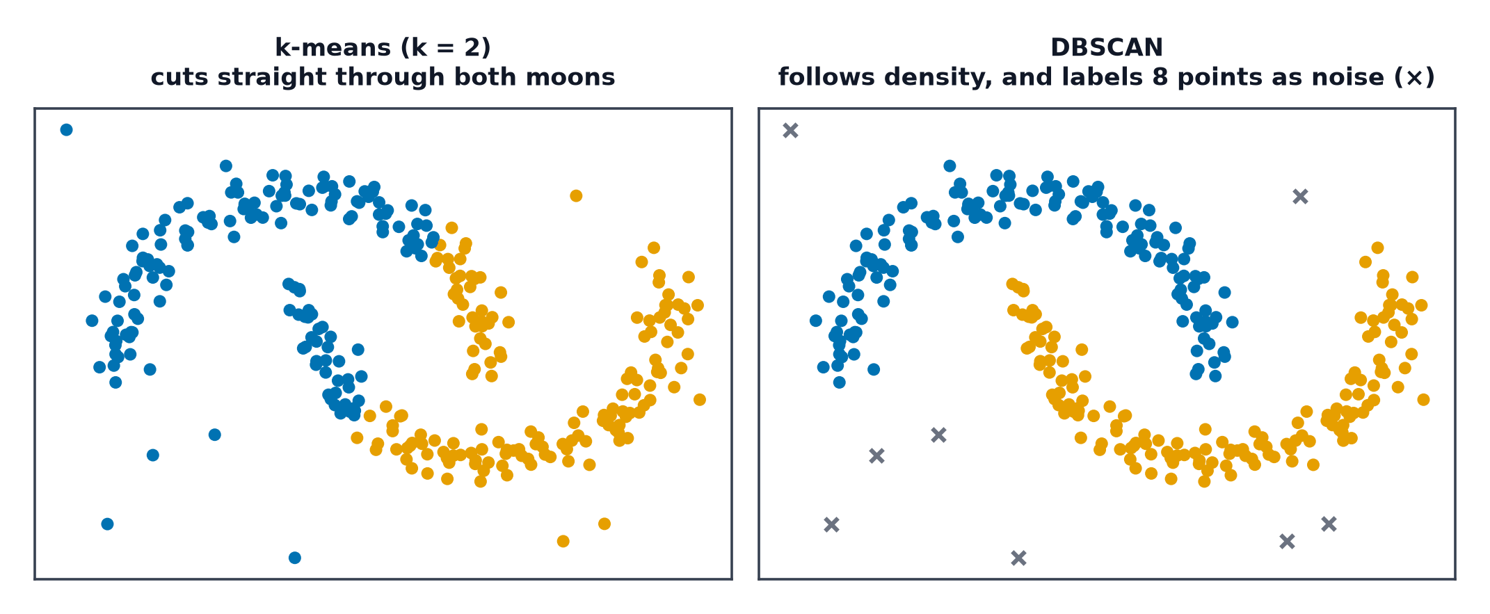
k-means needs to be told $k$ in advance, and assumes every cluster is roughly round. This page covers two families that relax those assumptions in different directions: hierarchical clustering defers the choice of cluster count to a visual cut, and density-based clustering abandons the "round cluster" assumption entirely by defining a cluster as a connected region of high density.

Key idea

Hierarchical clustering defers the choice of k to a dendrogram cut; density methods define clusters by connectivity, so shape stops mattering.

DBSCAN follows connected regions of high density, so it recovers the crescents k-means cannot — and it labels genuine outliers as noise rather than forcing every point into a cluster.

Agglomerative clustering

Start with every point as its own cluster; repeatedly merge the two closest clusters; stop when one cluster remains (or a target count is reached). The full sequence of merges is a dendrogram — a tree recording the order and distance of every merge.

Linkage criteria and the chaining effect

• Single linkage: distance between the closest pair of points across two clusters. Prone to the chaining effect — a thin bridge of points can merge two otherwise well-separated clusters, since only one close pair is needed.
• Complete linkage: distance between the farthest pair. Produces more compact, evenly-sized clusters, resists chaining.
• Average linkage: mean distance across all pairs. A middle ground.
• Ward's method: merges whichever pair minimises the resulting increase in within-cluster variance — tends to produce well-balanced clusters, similar in spirit to k-means' objective.

Reading a dendrogram

Hierarchical clustering produces the whole merge tree; you choose k afterwards by picking a cut height. The tall vertical gap just below the cut is the visual signal that two clusters is the natural answer here.

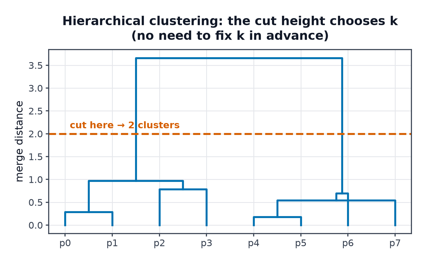
The height of each merge represents the distance at which it occurred. Cutting the dendrogram horizontally at a chosen height yields a clustering: every vertical line crossed by the cut becomes a separate cluster. A large vertical gap between two merge heights suggests a natural place to cut.

Divisive clustering, briefly

The reverse of agglomerative: start with one cluster, recursively split. Rarely used in practice — computationally more expensive than agglomerative merging.

Cost: O(n² log n), and what that rules out

Agglomerative clustering requires tracking pairwise distances across the whole dataset, which scales poorly — impractical much past tens of thousands of points without approximation.

DBSCAN: core, border, and noise points

DBSCAN defines clusters via local density rather than distance to a centroid:

• A core point has at least min_samples other points within radius eps.
• A border point is within eps of a core point but doesn't itself have enough neighbours to be core.
• A noise point belongs to neither — explicitly labelled as an outlier, not forced into a cluster.

Clusters are formed by connecting core points that are within eps of each other, plus their border points.

Symbol	Meaning
eps	the neighbourhood radius
min_samples	minimum neighbours (within eps) for a point to be core

Choosing eps with a k-distance plot

Plot, for each point, the distance to its $k$-th nearest neighbour ($k$ = min_samples), sorted ascending — the "elbow" in this curve is a reasonable choice for eps, marking the transition from dense-region distances to sparse-region distances.

DBSCAN's strengths and its weakness

Strengths: finds arbitrarily-shaped clusters (unlike k-means' round-cluster assumption), and explicitly identifies noise rather than forcing every point into a cluster. Weakness: a single global eps cannot handle clusters of substantially different densities — a value tuned for a dense cluster will merge sparse regions into noise, and vice versa.

HDBSCAN

Extends DBSCAN to handle varying density by building a hierarchy of clusterings across a range of density thresholds and extracting the most stable clusters — addresses DBSCAN's single-density limitation at the cost of more hyperparameters and complexity.

Comparison against k-means

	k-means	Hierarchical	DBSCAN
Needs $k$ upfront	yes	no (choose from dendrogram)	no
Cluster shape	round only	any (depends on linkage)	arbitrary
Handles noise/outliers	no, every point assigned	no	yes, explicit noise label
Scales to large $n$	well	poorly	reasonably, with spatial indexing

Code: dendrogram, DBSCAN on two-moons, k-distance plot

hierarchical_density_demo.py

import numpy as np
import matplotlib.pyplot as plt
from scipy.cluster.hierarchy import dendrogram, linkage
from sklearn.datasets import make_moons, make_circles
from sklearn.cluster import AgglomerativeClustering, DBSCAN
from sklearn.neighbors import NearestNeighbors

# --- Dendrogram ---
rng = np.random.default_rng(0)
X_small = rng.normal(size=(20, 2))
Z = linkage(X_small, method="ward")
plt.figure(figsize=(8, 4))
dendrogram(Z)
plt.savefig("dendrogram.png")

agg = AgglomerativeClustering(n_clusters=3, linkage="ward").fit(X_small)
print("agglomerative cluster sizes:", np.bincount(agg.labels_))

# --- DBSCAN on two-moons and concentric circles where k-means fails ---
X_moons, _ = make_moons(n_samples=300, noise=0.05, random_state=0)
X_circles, _ = make_circles(n_samples=300, noise=0.05, factor=0.5, random_state=0)

fig, axes = plt.subplots(1, 2, figsize=(10, 4))
for ax, X_fail, title in zip(axes, [X_moons, X_circles], ["two moons", "concentric circles"]):
    labels = DBSCAN(eps=0.2, min_samples=5).fit_predict(X_fail)
    ax.scatter(X_fail[:, 0], X_fail[:, 1], c=labels)
    ax.set_title(f"{title} (DBSCAN, -1 = noise)")
plt.savefig("dbscan_success.png")

# --- k-distance plot for choosing eps ---
k = 5
neighbors = NearestNeighbors(n_neighbors=k).fit(X_moons)
distances, _ = neighbors.kneighbors(X_moons)
k_distances = np.sort(distances[:, -1])
plt.figure()
plt.plot(k_distances)
plt.ylabel(f"{k}-th nearest neighbour distance")
plt.savefig("k_distance_plot.png")

DBSCAN should correctly separate both the two-moons and concentric-circles shapes that defeated k-means on the equivalent examples in k-Means Clustering — direct confirmation that density-based connectivity handles non-convex shapes k-means structurally cannot.

When to reach for this

Data size	hierarchical: small-to-moderate; DBSCAN: moderate-to-large with spatial indexing
Feature count	low-to-moderate; both degrade with the curse of dimensionality
Interpretability	hierarchical: high (dendrogram); DBSCAN: moderate
Training cost	hierarchical: $O(n^2 \log n)$; DBSCAN: $O(n \log n)$ with an index
Inference cost	DBSCAN has no native predict for new points; hierarchical likewise requires re-running

See also

• k-Means Clustering — the round-cluster baseline these methods extend beyond.
• Anomaly Detection — DBSCAN's noise label as an anomaly-detection signal.