k-Means Clustering

k-means is the clustering algorithm everyone reaches for first — and its simplicity conceals just how strong its assumptions are. It assumes clusters are round, similarly sized, and similarly dense, and it will happily produce a confident, wrong answer when those assumptions don't hold.

Key idea

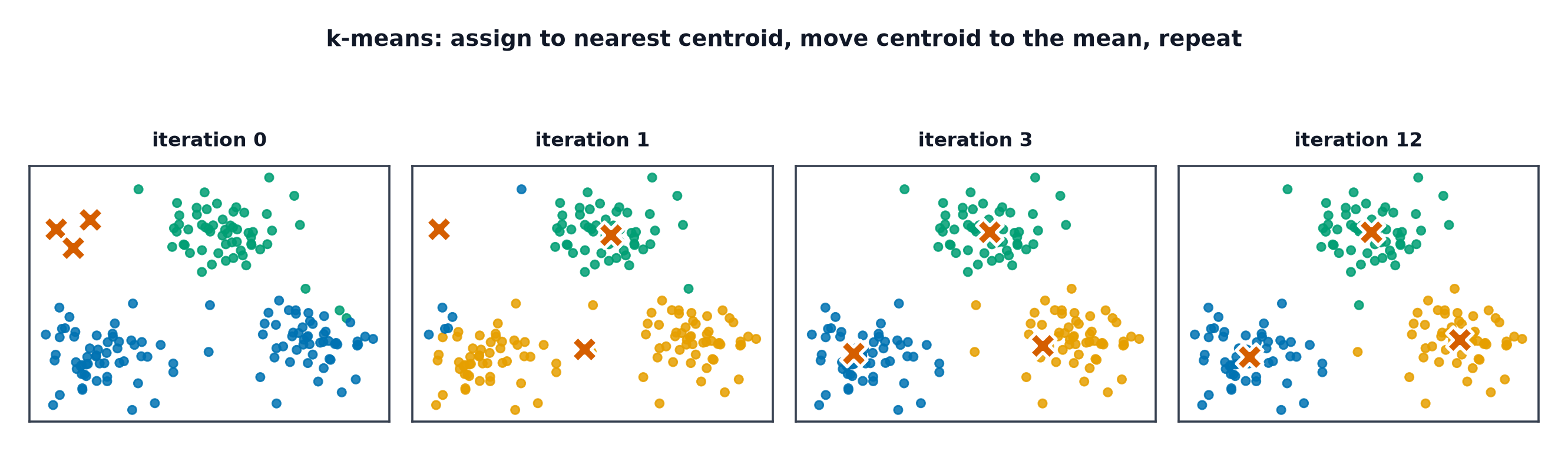
k-means alternates two trivial steps to minimise within-cluster variance — and in doing so assumes clusters are spherical, similarly sized, and equally dense.

k-means alternates two steps: assign each point to its nearest centroid, then move each centroid to the mean of its points. From this deliberately bad initialisation it still converges — but only to a local optimum, which is why k-means++ and restarts exist.

The objective

$$J = \sum_{i=1}^n \| x_i - \mu_{c_i} \|^2$$

Minimise the total squared distance from each point to its assigned cluster's centre — within-cluster sum of squares.

Symbol	Meaning
$c_i$	the cluster assigned to point $i$
$\mu_{c_i}$	the centroid of cluster $c_i$
$k$	number of clusters, chosen in advance

Lloyd's algorithm

1. Assign: put each point in the cluster of its nearest centroid.
2. Update: recompute each centroid as the mean of its assigned points.
3. Repeat until assignments stop changing.

Each step never increases $J$ (assignment picks the nearest centroid; update recomputes the mean, which minimises squared distance for a fixed assignment) — so the algorithm is guaranteed to converge, but only to a local optimum.

Convergence guarantees and local minima

Because $J$ is non-convex in the joint (assignment, centroid) space, different random starting points can converge to genuinely different final clusterings — there is no guarantee of finding the global optimum.

Initialisation matters: random vs. k-means++

Naive random initialisation can place initial centroids poorly, leading to slow convergence or a bad local optimum. k-means++ instead chooses initial centroids sequentially, each one selected with probability proportional to its squared distance from the nearest already-chosen centroid — spreading the initial centroids out and substantially improving both convergence speed and final quality.

Choosing k

k-means assumes roughly spherical, similarly sized clusters. Crescents and unequal spreads both defeat it. The elbow plot on the right is the standard heuristic for k — here bending cleanly at the true value of four.

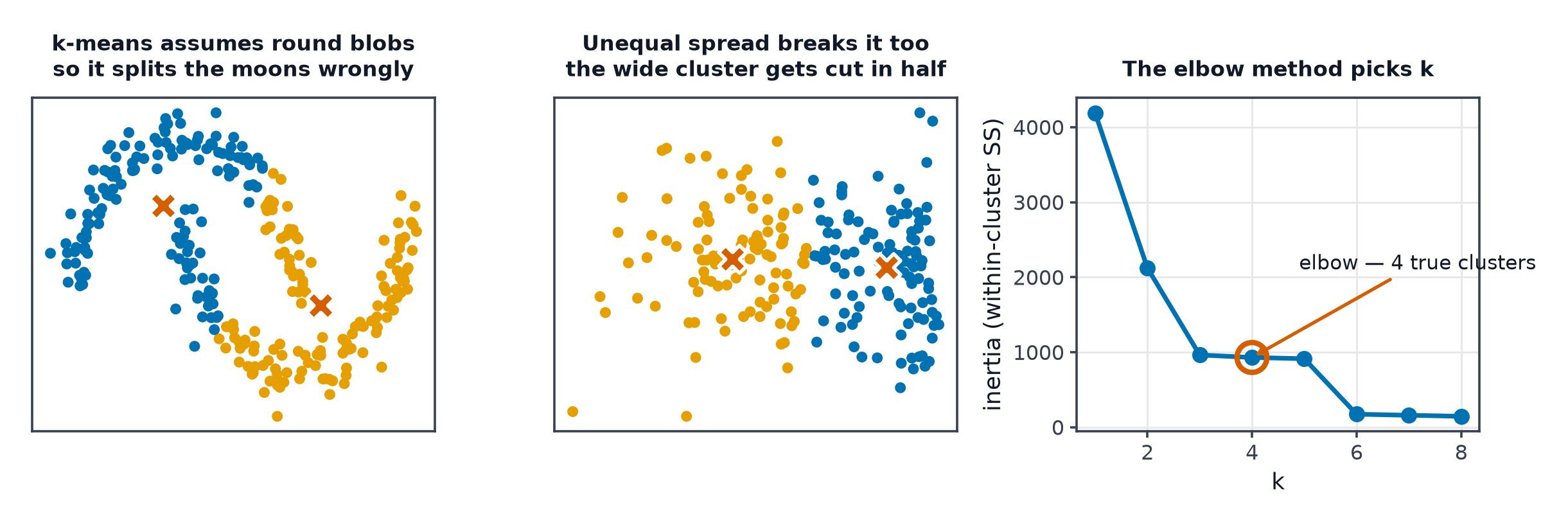
• Elbow method: plot $J$ against $k$; look for the point where the marginal decrease in $J$ sharply slows.
• Silhouette score: measures how similar each point is to its own cluster versus the nearest other cluster, averaged; higher is better.
• Gap statistic: compares $J$ against what would be expected under a null (uniform, no-cluster) reference distribution.

These three methods frequently disagree, especially on real (noisy, non-globular) data — treat them as suggestions, not a definitive answer.

Scaling is mandatory

k-means uses Euclidean distance directly, so an unscaled feature with a large numeric range will dominate cluster assignment — the same requirement as k-Nearest Neighbors and Support Vector Machines.

The assumptions, broken

• Elongated clusters: k-means assumes round (isotropic) clusters; an elongated cluster gets incorrectly split or merged with a neighbour.
• Unequal-size clusters: k-means tends to produce similarly-sized clusters even when the true clusters are very different sizes.
• Unequal-density clusters: a sparse large cluster and a dense small cluster nearby often get merged incorrectly.
• Non-convex clusters: two interlocking crescents (the "two moons" shape) cannot be correctly separated by any assignment based purely on distance to a single centroid per cluster.

Mini-batch k-means for scale

For very large datasets, computing centroids from the full dataset every iteration is expensive. Mini-batch k-means updates centroids using small random batches instead, trading a small amount of accuracy for a large speedup — the same batch-based idea as Gradient Descent.

k-means as vector quantisation

Beyond clustering for its own sake, k-means is used as a compression technique: replace every point with its cluster centroid, reducing a dataset (or an image's colour palette) to $k$ representative values.

Code: k-means from scratch with k-means++, four failure cases, elbow/silhouette

kmeans_demo.py

import numpy as np
import matplotlib.pyplot as plt
from sklearn.datasets import make_blobs, make_moons
from sklearn.cluster import KMeans
from sklearn.metrics import silhouette_score

def kmeans_plusplus_init(X, k, rng):
    centroids = [X[rng.integers(len(X))]]
    for _ in range(k - 1):
        dists = np.min([np.linalg.norm(X - c, axis=1) ** 2 for c in centroids], axis=0)
        probs = dists / dists.sum()
        centroids.append(X[rng.choice(len(X), p=probs)])
    return np.array(centroids)

def kmeans_fit(X, k, rng, max_iter=100):
    centroids = kmeans_plusplus_init(X, k, rng)
    for _ in range(max_iter):
        dists = np.linalg.norm(X[:, None] - centroids[None, :], axis=2)
        assignments = dists.argmin(axis=1)
        new_centroids = np.array([X[assignments == c].mean(axis=0) for c in range(k)])
        if np.allclose(new_centroids, centroids):
            break
        centroids = new_centroids
    return assignments, centroids

rng = np.random.default_rng(0)
X_blobs, _ = make_blobs(n_samples=300, centers=3, cluster_std=0.8, random_state=0)
assignments, centroids = kmeans_fit(X_blobs, k=3, rng=rng)
print("from-scratch k-means converged, cluster sizes:", np.bincount(assignments))

# --- Where k-means fails: elongated, unequal-density, non-convex ---
X_moons, _ = make_moons(n_samples=300, noise=0.05, random_state=0)
X_elongated = np.dot(np.random.default_rng(1).normal(size=(300, 2)), [[3, 0], [0, 0.3]])

fig, axes = plt.subplots(1, 2, figsize=(10, 4))
for ax, X_fail, title in zip(axes, [X_moons, X_elongated], ["two moons (non-convex)", "elongated"]):
    labels = KMeans(n_clusters=2, n_init=10, random_state=0).fit_predict(X_fail)
    ax.scatter(X_fail[:, 0], X_fail[:, 1], c=labels)
    ax.set_title(title)
plt.savefig("kmeans_failures.png")

# --- Elbow and silhouette on the well-suited blob data ---
inertias, sil_scores = [], []
for k in range(2, 8):
    km = KMeans(n_clusters=k, n_init=10, random_state=0).fit(X_blobs)
    inertias.append(km.inertia_)
    sil_scores.append(silhouette_score(X_blobs, km.labels_))
print("k=2..7 inertia:", np.round(inertias, 1))
print("k=2..7 silhouette:", np.round(sil_scores, 3), "  <- should peak near k=3, the true count")

When to reach for this

Data size	scales well, including with mini-batch variant
Feature count	works best after dimensionality reduction
Interpretability	high (centroids are directly inspectable)
Training cost	$O(nkd)$ per iteration
Inference cost	$O(kd)$ — distance to each centroid

See also

• Hierarchical and Density-Based Clustering — methods that handle the non-convex and unequal-density cases this one cannot.
• Gaussian Mixture Models — the soft-assignment, probabilistic generalisation of this algorithm.