k-Nearest Neighbors

Every model so far has fit parameters during training and thrown the raw data away afterward. kNN does the opposite: it stores the entire training set verbatim and defers all the actual work to inference time, where it asks "which stored examples look most like this new one?"

Key idea

kNN stores the training set and defers all work to inference — which makes it trivially flexible and hopeless at scale.

The algorithm

To classify a new point $x$: compute its distance to every training point, take the $k$ closest, and predict the majority class among them (or the average value, for regression).

Choosing k

k is the bias–variance dial made visible. At k = 1 every noisy point carves out its own island; at k = 75 the boundary is almost linear and the moons are lost. Nothing about the model changes but that one number.

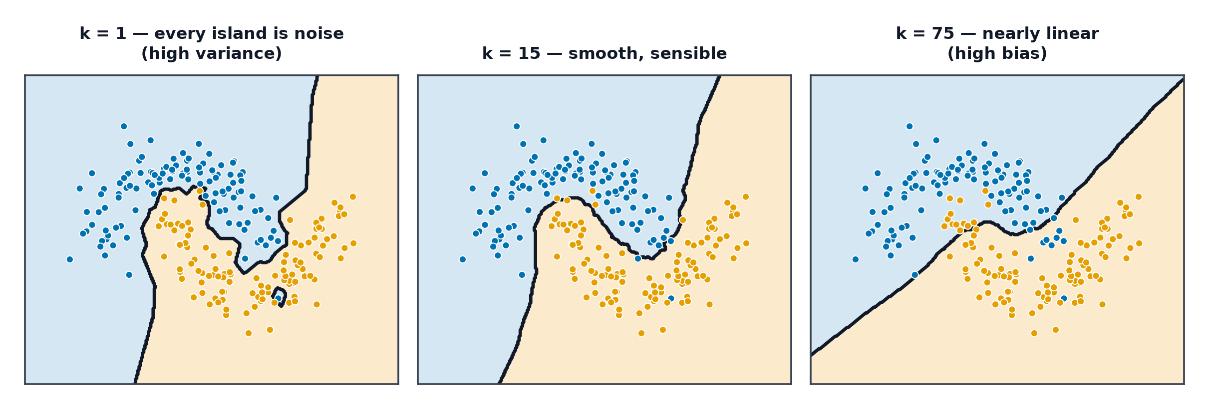
Small $k$ (e.g. $k=1$) fits the local structure tightly — low bias, high variance, sensitive to noise (a single mislabelled neighbour flips the prediction). Large $k$ smooths the decision boundary — higher bias, lower variance. This is the Bias-Variance Tradeoff made directly visible by a single hyperparameter.

Distance metrics

• Euclidean: $\sqrt{\sum_i (x_i - y_i)^2}$ — the default, sensitive to feature scale.
• Manhattan: $\sum_i |x_i - y_i|$ — less sensitive to outlier dimensions.
• Cosine: $1 - \frac{x \cdot y}{\|x\|\|y\|}$ — measures angle, not magnitude; standard for text and embeddings.
• Hamming: fraction of differing positions — for categorical or binary features.

Feature scaling is not optional

Distance metrics are dominated by whichever feature has the largest numeric range — a feature measured in thousands (income) will swamp one measured in single digits (age) unless both are standardised first (Data Preprocessing and Features).

Weighted voting

Instead of an unweighted majority vote among the $k$ neighbours, weight each neighbour's vote by the inverse of its distance — closer neighbours count more, which softens the effect of choosing $k$ slightly too large.

kNN for regression

The same algorithm, predicting the (weighted) average of the $k$ neighbours' target values instead of a majority vote.

Computational cost and approximate methods

A naive query is $O(nd)$ — compare against every training point. KD-trees and ball trees organise the training set spatially to prune most comparisons, reducing average query cost to roughly $O(\log n \cdot d)$ in low dimensions — but their advantage evaporates in high dimensions, where nearly every point ends up needing to be checked anyway (see below). For truly large-scale settings, approximate nearest neighbour methods (e.g. HNSW, used throughout vector-store retrieval) trade a small amount of accuracy for large speedups.

Symbol	Meaning
$k$	number of neighbours consulted
$n$	number of training points
$d$	number of features

The curse of dimensionality hits kNN hardest

As shown in Curse of Dimensionality, pairwise distances converge toward a single value as dimension grows — which means "the $k$ nearest points" stops being meaningfully different from "$k$ arbitrary points" once dimensionality is high. kNN is the algorithm most directly and severely damaged by this effect.

Code: kNN from scratch, boundary comparison, timing against sklearn

knn_demo.py

import time
import numpy as np
import matplotlib.pyplot as plt
from sklearn.datasets import make_moons
from sklearn.neighbors import KNeighborsClassifier

def knn_predict(X_train, y_train, X_query, k):
    preds = np.zeros(len(X_query), dtype=int)
    for i, q in enumerate(X_query):
        dists = np.linalg.norm(X_train - q, axis=1)  # vectorised Euclidean distance
        nearest = np.argsort(dists)[:k]
        preds[i] = np.bincount(y_train[nearest]).argmax()
    return preds

X, y = make_moons(n_samples=300, noise=0.25, random_state=0)

xx, yy = np.meshgrid(np.linspace(X[:, 0].min()-0.5, X[:, 0].max()+0.5, 100),
                      np.linspace(X[:, 1].min()-0.5, X[:, 1].max()+0.5, 100))
grid = np.c_[xx.ravel(), yy.ravel()]

fig, axes = plt.subplots(1, 3, figsize=(15, 4))
for ax, k in zip(axes, [1, 5, 50]):
    preds = knn_predict(X, y, grid, k).reshape(xx.shape)
    ax.contourf(xx, yy, preds, alpha=0.4)
    ax.scatter(X[:, 0], X[:, 1], c=y, edgecolors="k", s=15)
    ax.set_title(f"k={k}")
plt.savefig("knn_boundaries.png")

# --- Timing: hand-written vs sklearn's tree-based backend ---
start = time.perf_counter()
knn_predict(X, y, grid[:500], k=5)
print(f"hand-written (brute force): {time.perf_counter() - start:.4f}s")

sk_knn = KNeighborsClassifier(n_neighbors=5).fit(X, y)
start = time.perf_counter()
sk_knn.predict(grid[:500])
print(f"sklearn (tree-based):       {time.perf_counter() - start:.4f}s")

At $k=1$ the boundary hugs every training point tightly (jagged, high variance); at $k=50$ it smooths into a much simpler shape (higher bias) — the same tradeoff described above, made visible.

When to reach for this

Data size	small-to-moderate — no separate training cost, but query cost scales with $n$
Feature count	low, ideally after dimensionality reduction
Interpretability	high (can inspect the actual neighbours)
Training cost	effectively zero (just stores the data)
Inference cost	high, $O(nd)$ per query without a spatial index

See also

• Curse of Dimensionality — why this algorithm degrades fastest in high dimensions.
• Data Preprocessing and Features — the scaling step this algorithm cannot skip.