Kernel Methods

Some data simply cannot be separated by a straight line — two concentric circles of different classes have no linear boundary at all. The kernel trick lets a linear algorithm operate as if the data had been lifted into a much higher-dimensional (sometimes infinite-dimensional) space where a linear boundary does exist, without ever actually computing that lift.

Key idea

Any algorithm written purely in terms of dot products can swap that dot product for a kernel and gain a non-linear boundary for free.

The kernel trick in one picture. Data that needs a circular boundary in 2-D needs only a flat plane once lifted by a radial feature — and the kernel computes the inner products in that higher space without ever building it.

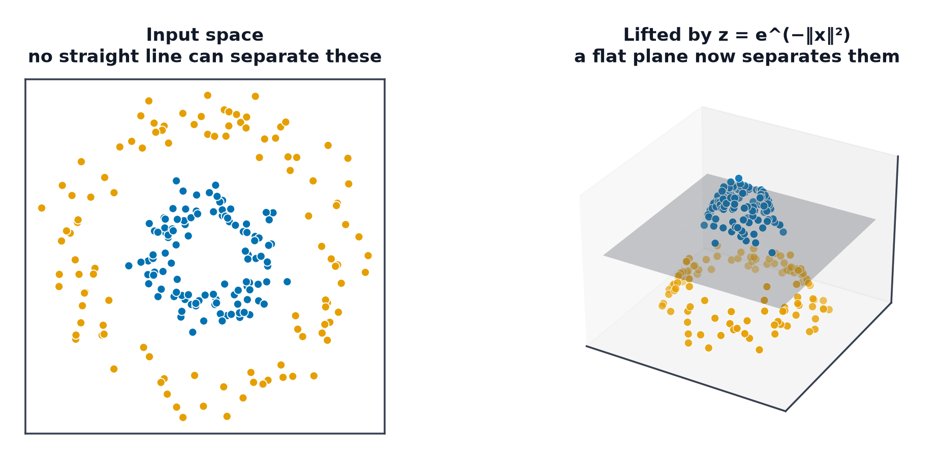
The problem: non-linearly-separable data

Concentric circles, XOR-like patterns, spirals — data where no hyperplane in the original feature space separates the classes.

Explicit feature maps and their cost

One fix: manually engineer non-linear features (e.g. $\phi(x) = (x_1, x_2, x_1^2, x_2^2, x_1 x_2)$) and run a linear method on those. This works, but the required feature map can be astronomically high-dimensional (or infinite-dimensional, as with the RBF kernel below) — computing $\phi(x)$ explicitly is often infeasible.

The kernel trick

Support Vector Machines's dual formulation depends on the data only through pairwise dot products $x_i \cdot x_j$. The kernel trick replaces that dot product with a kernel function $K(x, x') = \langle \phi(x), \phi(x') \rangle$ that computes the dot product in the higher-dimensional space directly from the original inputs — without ever materialising $\phi(x)$:

$$K(x, x') = \langle \phi(x), \phi(x') \rangle$$

Symbol	Meaning
$\phi$	the (possibly infeasible-to-compute) implicit feature map
$K(x, x')$	the kernel function, computed directly from $x, x'$
$\gamma$	the RBF kernel's bandwidth parameter

Mercer's condition

Not every function $K$ is a valid kernel — it must correspond to some actual dot product in some feature space. Mercer's condition (roughly: $K$ must be positive semi-definite) is the mathematical guarantee that a proposed $K$ has this property.

The standard kernels

• Linear: $K(x,x') = x \cdot x'$ — equivalent to no kernel at all.
• Polynomial: $K(x,x') = (x \cdot x' + c)^p$ — implicitly includes all feature interactions up to degree $p$.
• RBF/Gaussian: $K(x,x') = e^{-\gamma\|x-x'\|^2}$ — corresponds to an infinite-dimensional feature space; the most commonly used non-linear kernel.
• Sigmoid: $K(x,x') = \tanh(\alpha x \cdot x' + c)$ — occasionally used, behaves similarly to a neural network's single layer.

What gamma controls in RBF

$\gamma$ sets how far a single training point's influence reaches — large $\gamma$ means influence decays quickly with distance (a tight, wiggly boundary, prone to overfitting), small $\gamma$ means influence extends far (a smooth, near-linear boundary, prone to underfitting).

The C/gamma grid and its overfitting corner

Sweeping both $C$ (margin cost, from Support Vector Machines) and $\gamma$ together reveals a characteristic region — large $C$ combined with large $\gamma$ — where validation accuracy collapses even as training accuracy stays near-perfect, the signature of severe overfitting from a boundary that wraps tightly around individual training points.

Kernels beyond SVM

The same trick applies wherever an algorithm is expressed purely via dot products: kernel ridge regression and kernel PCA (PCA and SVD) both gain non-linear power the identical way.

Cost: the Gram matrix, and why kernels lost to deep nets on large data

Computing $K(x_i, x_j)$ for every pair of $n$ training points produces an $n \times n$ Gram matrix — $O(n^2)$ memory and typically $O(n^2)$–$O(n^3)$ compute to train on it. This scales badly past tens of thousands of examples, which is a major reason kernel methods lost ground to deep neural networks (whose cost scales with parameters and data linearly per pass, not quadratically with dataset size) once datasets grew into the millions.

Code: linear/poly/RBF boundaries, and the overfitting grid

kernel_methods_demo.py

import numpy as np
import matplotlib.pyplot as plt
from sklearn.svm import SVC
from sklearn.datasets import make_circles
from sklearn.model_selection import GridSearchCV

X, y = make_circles(n_samples=200, noise=0.1, factor=0.3, random_state=0)

fig, axes = plt.subplots(1, 3, figsize=(15, 4))
xx, yy = np.meshgrid(np.linspace(-1.5, 1.5, 200), np.linspace(-1.5, 1.5, 200))
for ax, kernel in zip(axes, ["linear", "poly", "rbf"]):
    model = SVC(kernel=kernel, degree=3).fit(X, y)
    Z = model.predict(np.c_[xx.ravel(), yy.ravel()]).reshape(xx.shape)
    ax.contourf(xx, yy, Z, alpha=0.4)
    ax.scatter(X[:, 0], X[:, 1], c=y, edgecolors="k")
    ax.set_title(kernel)
plt.savefig("kernel_boundaries.png")

# --- C x gamma grid, showing the overfit corner ---
param_grid = {"C": [0.1, 1, 10, 100], "gamma": [0.01, 0.1, 1, 10]}
grid = GridSearchCV(SVC(kernel="rbf"), param_grid, cv=5)
grid.fit(X, y)
scores = grid.cv_results_["mean_test_score"].reshape(4, 4)
print("validation accuracy grid (rows=C, cols=gamma):")
print(np.round(scores, 3))

Only the RBF kernel should produce a boundary that correctly separates the concentric circles — linear and (low-degree) polynomial kernels cannot, no matter how they're tuned, since no straight or mildly-curved line separates two nested circles.

When to reach for this

Data size	small-to-moderate (Gram matrix cost)
Feature count	works well in low-to-moderate dimensions with genuine non-linear structure
Interpretability	low — the implicit feature space isn't directly inspectable
Training cost	$O(n^2)$–$O(n^3)$
Inference cost	proportional to number of support vectors

See also

• Support Vector Machines — the dual formulation this trick plugs into.
• PCA and SVD — kernel PCA, the unsupervised analogue.