Linear Regression

Every model in this knowledge base is measured against linear regression, and for good reason: it's the only widely-used model whose optimum you can write down in one line, no iteration required. Understanding exactly why that's possible — and exactly when it stops being possible — is the fastest way to understand the rest of classical ML.

Key idea

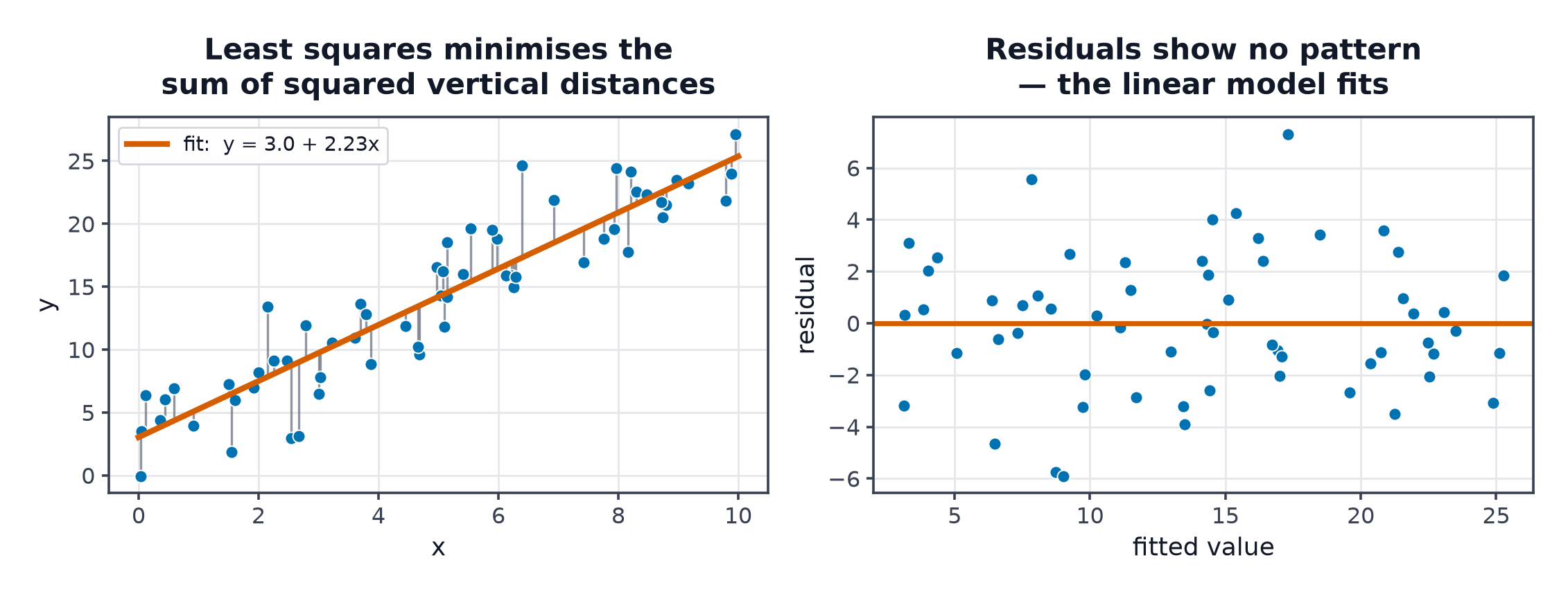
Fitting a line is solving a convex least-squares problem — there is exactly one answer, and you can write it down in closed form.

Least squares minimises the sum of the squared vertical distances — the grey segments. Squaring is what makes distant points dominate the fit, and why a single outlier can tilt the whole line.

The model

$$\hat y = Xw + b$$

Each prediction is a weighted sum of features plus a bias term. In matrix form, absorbing $b$ into $w$ by adding a constant column of ones to $X$, this is just $\hat y = Xw$.

Least squares objective

$$L(w) = \frac{1}{n}\|Xw - y\|_2^2 = \frac{1}{n}\sum_i (x_i^\top w - y_i)^2$$

This is exactly the MSE loss from Loss Functions, and it is convex in $w$ — a single global minimum, no local minima to worry about.

The normal equation, derived

Setting the gradient to zero:

$$\nabla_w L(w) = \frac{2}{n}X^\top(Xw - y) = 0 \;\Rightarrow\; X^\top X w = X^\top y \;\Rightarrow\; w^* = (X^\top X)^{-1}X^\top y$$

Symbol	Meaning
$X$	design matrix, one row per example, one column per feature (plus a bias column)
$w$	weight vector
$y$	targets
$(X^\top X)^{-1}X^\top$	the pseudo-inverse of $X$, from Linear Algebra

Why gradient descent is still used

The normal equation requires inverting $X^\top X$, a $d \times d$ matrix — cost $O(d^3)$. For millions of features, or when $X^\top X$ is singular (perfectly collinear features), the closed form is infeasible or undefined, and Gradient Descent becomes the practical choice.

Assumptions and what breaks when they fail

Anscombe's quartet: four datasets with identical means, variances, correlation and regression line. Summary statistics alone cannot tell them apart — which is the entire argument for plotting your data first.

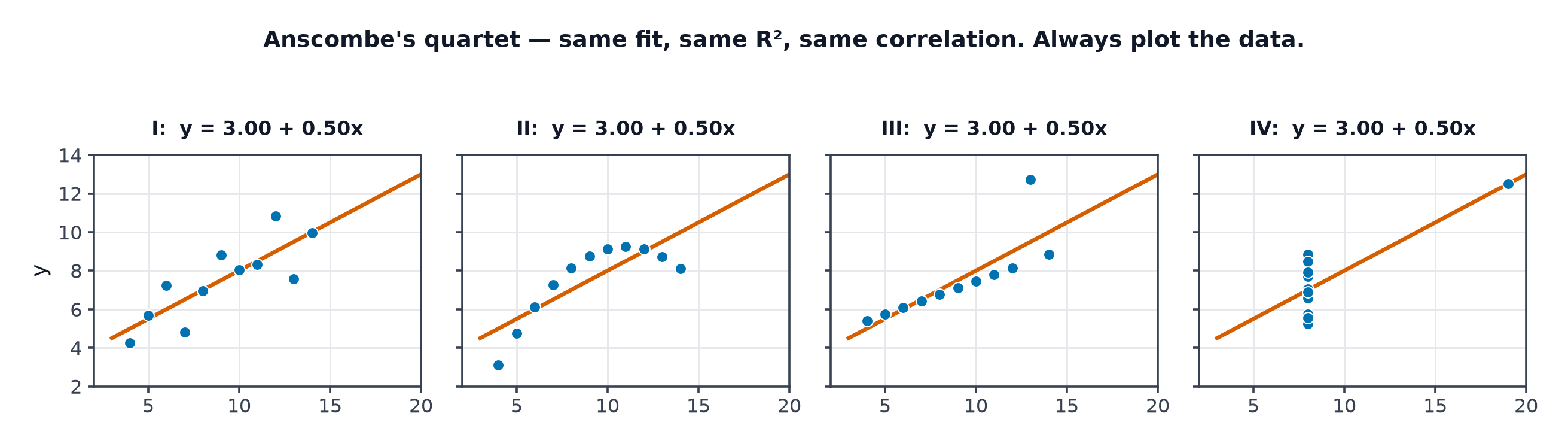
• Linearity: the true relationship is (approximately) linear in the features — fails on curved relationships, fixed by polynomial features below.
• Independence: errors aren't correlated across examples — fails for time series with autocorrelated residuals.
• Homoscedasticity: constant error variance — fails when noise grows with the magnitude of $y$ (visible as a funnel in a residual plot, see Evaluation Metrics for Regression).
• Normal residuals: needed for classical confidence intervals on coefficients, not for the point estimate itself.

Multicollinearity and the condition number

When features are highly correlated, $X^\top X$ is nearly singular — its inverse becomes numerically unstable, and small changes in the data produce wildly different coefficient estimates even though predictions barely change. The condition number of $X^\top X$ (ratio of largest to smallest eigenvalue) quantifies this instability; Regularization: Ridge, Lasso, Elastic Net is the standard fix.

Polynomial and basis expansion

Linear regression on engineered features $[x, x^2, x^3, \ldots]$ can fit curves while the model itself remains linear in its parameters — the "linear" in linear regression refers to linearity in $w$, not in $x$.

Interpreting coefficients (and the units trap)

A coefficient $w_i$ says "holding all other features fixed, a one-unit increase in feature $i$ changes $\hat y$ by $w_i$." The trap: comparing raw coefficient magnitudes across features with different units (dollars vs. years) is meaningless — standardise features first if you want to compare their relative importance.

Residual diagnostics

Plot residuals against fitted values and against each feature. A random scatter around zero confirms the assumptions; a curved pattern means missing non-linearity; a funnel shape means heteroscedasticity.

Code: normal equation vs. gradient descent, and multicollinearity's instability

linear_regression_demo.py

import numpy as np
from sklearn.linear_model import LinearRegression

rng = np.random.default_rng(0)
n, d = 200, 3
X = rng.normal(size=(n, d))
true_w = np.array([2.0, -1.0, 0.5])
y = X @ true_w + rng.normal(scale=0.1, size=n)

# --- Normal equation ---
X_bias = np.hstack([X, np.ones((n, 1))])
w_closed = np.linalg.pinv(X_bias.T @ X_bias) @ X_bias.T @ y
print("normal equation weights (+bias):", w_closed)

# --- Gradient descent ---
def gd_fit(X, y, lr=0.05, steps=500):
    w = np.zeros(X.shape[1])
    for _ in range(steps):
        w -= lr * (2 / len(y)) * X.T @ (X @ w - y)
    return w

w_gd = gd_fit(X_bias, y)
print("gradient descent weights (+bias):", w_gd, "  <- should match normal equation")

# --- sklearn, for comparison ---
sk_model = LinearRegression().fit(X, y)
print("sklearn:", sk_model.coef_, sk_model.intercept_)

# --- Multicollinearity: near-duplicate features destabilise coefficients ---
X_collinear = np.hstack([X, X[:, [0]] + rng.normal(scale=1e-3, size=(n, 1))])  # near-copy of col 0
for trial in range(3):
    noise = rng.normal(scale=1e-4, size=X_collinear.shape)
    w_unstable = np.linalg.pinv((X_collinear + noise).T @ (X_collinear + noise)) @ (X_collinear + noise).T @ y
    print(f"trial {trial}, tiny perturbation -> coefficients: {w_unstable}")

The multicollinearity block is the point: adding a near-duplicate column and perturbing the data by a tiny amount produces wildly different coefficient estimates each trial — direct evidence of the instability, even though predictions on held-out data barely change.

When to reach for this

Data size	any, scales well
Feature count	low-to-moderate without regularisation, any with it
Interpretability	highest of any model family
Training cost	$O(d^3)$ closed form, or cheap with gradient descent
Inference cost	one dot product — essentially free

See also

• Gradient Descent — the iterative alternative to the closed form.
• Regularization: Ridge, Lasso, Elastic Net — the fix for multicollinearity and overfitting.