Logistic Regression

Despite the name, logistic regression is a classifier, and it remains the first model worth trying on any new tabular classification task — fast to train, easy to interpret, and a strong baseline against which everything fancier should be measured.

Key idea

It is a linear model on the log-odds — the sigmoid only converts that line into a probability.

The sigmoid turns an unbounded score into a probability. The boundary it produces is always linear in the input features — the curve is in the probability, not in the separator.

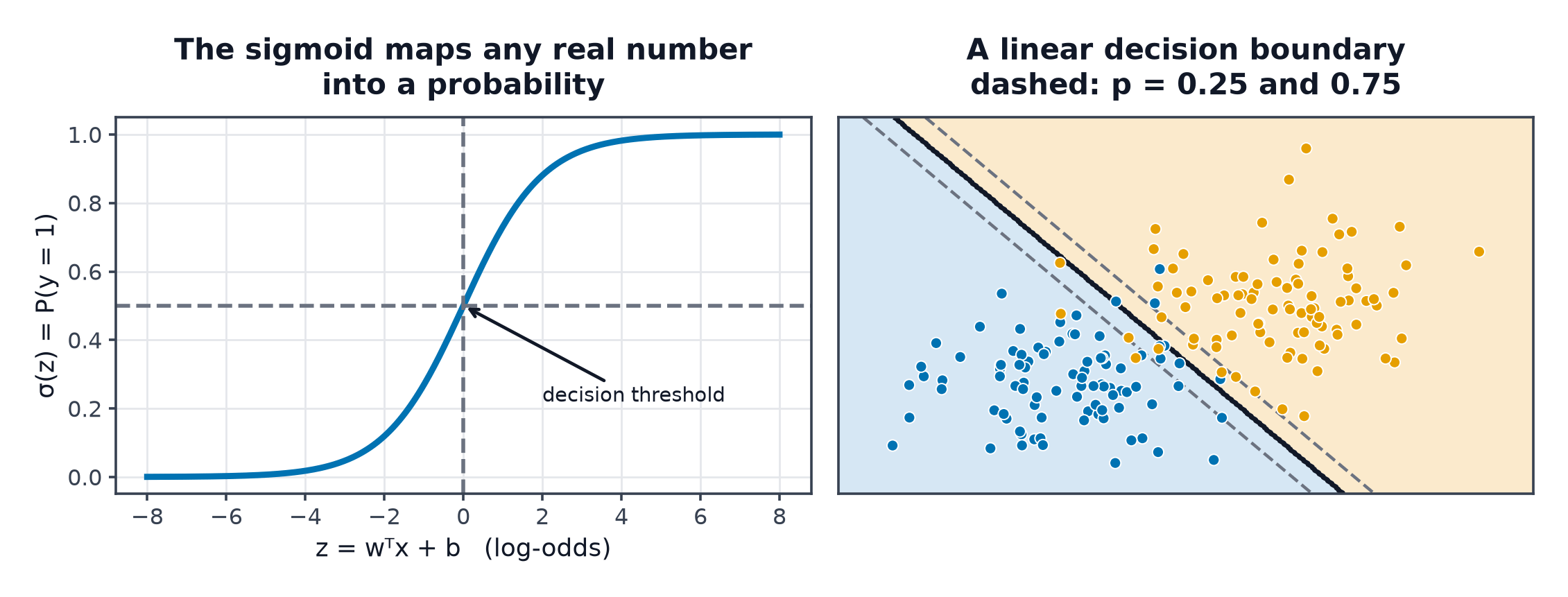
Why linear regression fails for classification

Fitting $\hat y = Xw$ directly to 0/1 labels produces predictions outside $[0,1]$, and squared error penalises a wildly wrong confident prediction the same way it penalises a mild one — the wrong loss for a probability.

The sigmoid

$$\sigma(z) = \frac{1}{1+e^{-z}}$$

Squashes any real number into $(0, 1)$, monotonically, with a characteristic S-curve — exactly what's needed to turn an unbounded linear score into a probability.

Log-odds and the linear decision boundary

Logistic regression models the log-odds as linear in the features:

$$\log\frac{p}{1-p} = Xw \;\Leftrightarrow\; p = \sigma(Xw)$$

The decision boundary ($p = 0.5$, i.e. $Xw = 0$) is a straight line (or hyperplane) — logistic regression is still a linear classifier, just with a non-linear link function connecting the linear score to a probability.

The likelihood and cross-entropy

Assuming labels are Bernoulli with $p(y=1|x) = \sigma(x^\top w)$, the negative log-likelihood over the dataset is exactly binary cross-entropy from Loss Functions — this is the Statistics and Estimation MLE-to-loss bridge made concrete for classification.

No closed form: gradient descent and Newton/IRLS

Unlike linear regression, there's no algebraic solution — the loss is convex but transcendental. Gradient descent works; Newton's method (iteratively reweighted least squares, IRLS) converges faster by using second-order curvature information, at higher cost per step.

The gradient, derived

$$\nabla_w L(w) = X^\top(\sigma(Xw) - y)$$

Symbol	Meaning
$\sigma(z)$	the sigmoid function
$X, w, y$	design matrix, weights, binary labels
$\sigma(Xw) - y$	the prediction error vector

Remarkably, this has the identical form to linear regression's gradient $X^\top(Xw - y)$ — the "prediction minus target" pattern recurs throughout this knowledge base because both are instances of the same generalised linear model framework.

Multi-class: softmax and one-vs-rest

For $K > 2$ classes: softmax regression generalises the sigmoid to $p_k = \frac{e^{z_k}}{\sum_j e^{z_j}}$ over $K$ linear scores simultaneously (see Attention Mechanism for softmax's other major use). One-vs-rest instead trains $K$ independent binary classifiers, each distinguishing one class from all others — simpler, occasionally less calibrated.

Interpreting coefficients as odds ratios

$e^{w_i}$ is the multiplicative change in odds ($p/(1-p)$) for a one-unit increase in feature $i$ — a coefficient of $w_i = 0.69$ means the odds roughly double ($e^{0.69} \approx 2$) per unit increase.

Regularised variants

L1/L2 penalties apply identically to logistic regression's loss as they do to linear regression's — see Regularization: Ridge, Lasso, Elastic Net.

Calibration

Because the training objective is a proper probabilistic likelihood, logistic regression tends to produce well-calibrated probabilities out of the box — a genuine advantage over models like SVMs or random forests, whose outputs require separate calibration if probabilities (not just labels) matter downstream.

Code: gradient descent from scratch, matched against sklearn

logistic_regression_demo.py

import numpy as np
from sklearn.linear_model import LogisticRegression
from sklearn.datasets import make_classification
import matplotlib.pyplot as plt

def sigmoid(z):
    return 1 / (1 + np.exp(-z))

def fit_logistic_gd(X, y, lr=0.1, steps=2000):
    X_bias = np.hstack([X, np.ones((len(X), 1))])
    w = np.zeros(X_bias.shape[1])
    for _ in range(steps):
        grad = X_bias.T @ (sigmoid(X_bias @ w) - y) / len(y)
        w -= lr * grad
    return w

X, y = make_classification(n_samples=300, n_features=2, n_redundant=0, n_informative=2,
                            n_clusters_per_class=1, random_state=0)

w_scratch = fit_logistic_gd(X, y)
sk_model = LogisticRegression().fit(X, y)

print("from scratch (weights, bias):", w_scratch)
print("sklearn (weights, bias):     ", sk_model.coef_[0], sk_model.intercept_[0])

# --- Decision boundary plot ---
xx, yy = np.meshgrid(np.linspace(X[:, 0].min(), X[:, 0].max(), 200),
                      np.linspace(X[:, 1].min(), X[:, 1].max(), 200))
grid = np.c_[xx.ravel(), yy.ravel()]
probs = sk_model.predict_proba(grid)[:, 1].reshape(xx.shape)

fig, ax = plt.subplots()
ax.contourf(xx, yy, probs, levels=20, alpha=0.6)
ax.scatter(X[:, 0], X[:, 1], c=y, edgecolors="k")
plt.savefig("logistic_boundary.png")

The scratch-built weights and sklearn's should closely agree, confirming the hand-derived gradient is correct.

When to reach for this

Data size	any, including small
Feature count	low-to-moderate, or high with L1/L2
Interpretability	very high (odds-ratio coefficients)
Training cost	fast, convex, converges reliably
Inference cost	one dot product plus a sigmoid — essentially free

See also

• Information Theory — cross-entropy, the loss this model minimises.
• Evaluation Metrics for Classification — how to evaluate the resulting classifier properly.