Manifold Learning

t-SNE and UMAP produce the 2-D scatter plots of high-dimensional embeddings that appear everywhere — clusters of colourful dots, each supposedly a meaningful group. They are genuinely useful, and also genuinely easy to misread: knowing exactly what these plots do and do not preserve is the difference between a real insight and a confident misinterpretation.

Key idea

t-SNE and UMAP preserve local neighbourhoods, not global geometry; cluster sizes and inter-cluster distances in the output are largely meaningless.

Points close in Euclidean distance can be far apart along the manifold — the two facing surfaces of the roll are adjacent in 3-D but distant along the sheet. Manifold learning recovers the intrinsic coordinates on the right.

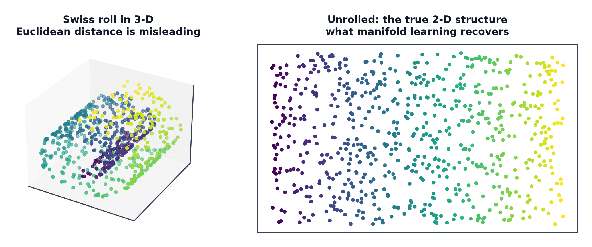
Why linear projection fails on curved manifolds

PCA and SVD can only find linear combinations of features. If the true structure of the data is a curved, lower-dimensional surface embedded in a high-dimensional space (imagine a rolled-up sheet of paper in 3-D), a linear projection will cut straight through the curve rather than "unrolling" it — points that are far apart along the manifold's surface can end up projected close together.

The manifold hypothesis

Real high-dimensional data (images, embeddings) is believed to lie near a much lower-dimensional curved manifold within the ambient space, not spread uniformly through it — the same hypothesis underlying Curse of Dimensionality's discussion of why deep networks cope with high-dimensional inputs. Manifold learning methods try to recover that lower-dimensional structure directly.

t-SNE: pairwise similarities, the Student-t tail, KL objective

t-SNE converts high-dimensional pairwise distances into conditional probabilities $p_{j|i}$ (a Gaussian kernel around each point) and low-dimensional pairwise distances into probabilities $q_{ij}$ (using a heavy-tailed Student-t distribution instead of a Gaussian). It then minimises the KL divergence between the two:

$$D_{KL}(P \parallel Q) = \sum_{i \ne j} p_{ij} \log \frac{p_{ij}}{q_{ij}}$$

The heavy Student-t tail in the low-dimensional space is deliberate: it lets moderately-distant points in the low-dimensional embedding correspond to a wider range of high-dimensional distances, which counteracts the tendency of naive embeddings to crowd everything into the centre (the "crowding problem").

Symbol	Meaning
$p_{j \mid i}$	high-dimensional conditional similarity of point $j$ to point $i$
$q_{ij}$	low-dimensional similarity in the embedding
perplexity	roughly, the effective number of neighbours considered per point

Perplexity

t-SNE's main hyperparameter controls the effective neighbourhood size used to compute $p_{j|i}$. Different perplexity values can produce visibly different cluster structure from the same data — a low perplexity emphasises very local structure (small, tight sub-clusters), a high perplexity emphasises broader groupings. There is no single "correct" perplexity; running a few values is standard practice.

t-SNE's non-determinism and non-parametric nature

Two runs with different random initialisations can produce visually different (though often qualitatively similar) layouts. And t-SNE has no transform method for new points — the entire embedding must be recomputed from scratch if new data arrives, unlike PCA's simple linear projection.

UMAP: topological motivation, speed, hyperparameters

UMAP is grounded in a different mathematical framework (fuzzy topological structure) but pursues a similar goal — preserve local neighbourhood structure in a lower-dimensional embedding. In practice it is substantially faster than t-SNE on large datasets and tends to better preserve some aspects of global structure. Its two main hyperparameters: n_neighbors (analogous to perplexity — local vs. global emphasis) and min_dist (how tightly points are allowed to pack together in the embedding).

What you may and may not conclude from these plots

May conclude: points that appear close together in the embedding were probably close together (in a local-neighbourhood sense) in the original space. May not conclude: that the size of a visual cluster reflects how many points are truly similar, that the distance between two clusters reflects how dissimilar those groups are, or that a shape (a ring, a branch) in the embedding corresponds to a genuine geometric structure in the original data — all three are common misreadings that these algorithms' local-preservation objective does not support.

Comparison against PCA

	PCA	t-SNE / UMAP
Preserves	global variance, linear structure	local neighbourhoods only
Deterministic	yes	t-SNE: no; UMAP: mostly
Transform for new points	yes, trivially	t-SNE: no; UMAP: approximately
Interpretation of distances	meaningful	not meaningful beyond local neighbourhoods
Speed	fast	UMAP: moderate; t-SNE: slow on large data

Practical recipe: PCA first, then t-SNE/UMAP

Running t-SNE or UMAP directly on very high-dimensional data (thousands of raw features) is slow and noisy. Standard practice: reduce to ~50 dimensions with PCA first (fast, removes noise dimensions), then apply t-SNE or UMAP to those 50 dimensions for the final 2-D visualisation.

Code: t-SNE at three perplexities, PCA for contrast

manifold_learning_demo.py

import matplotlib.pyplot as plt
from sklearn.datasets import load_digits
from sklearn.decomposition import PCA
from sklearn.manifold import TSNE

digits = load_digits()
X, y = digits.data, digits.target

fig, axes = plt.subplots(1, 4, figsize=(16, 4))

# --- PCA, for contrast ---
X_pca = PCA(n_components=2).fit_transform(X)
axes[0].scatter(X_pca[:, 0], X_pca[:, 1], c=y, cmap="tab10", s=8)
axes[0].set_title("PCA (linear, global variance)")

# --- t-SNE at three perplexities: the same data, visibly different pictures ---
for ax, perplexity in zip(axes[1:], [5, 30, 100]):
    X_tsne = TSNE(n_components=2, perplexity=perplexity, random_state=0, init="pca").fit_transform(X)
    ax.scatter(X_tsne[:, 0], X_tsne[:, 1], c=y, cmap="tab10", s=8)
    ax.set_title(f"t-SNE, perplexity={perplexity}")

plt.savefig("manifold_comparison.png")

The three t-SNE panels, run on the identical dataset, should look visibly different from each other — direct evidence that perplexity is not a cosmetic setting but a real change in what local structure the embedding emphasises.

When to reach for this

Data size	moderate; t-SNE scales poorly past tens of thousands of points, UMAP better
Feature count	any, ideally pre-reduced with PCA to ~50
Interpretability	visualisation only — do not use embedding distances as a downstream feature
Training cost	UMAP: moderate; t-SNE: slow, especially at scale
Inference cost	UMAP: approximate transform available; t-SNE: none, must rerun

See also

• PCA and SVD — the linear method these algorithms extend beyond.
• Curse of Dimensionality — the manifold hypothesis motivating this whole family.