Naive Bayes

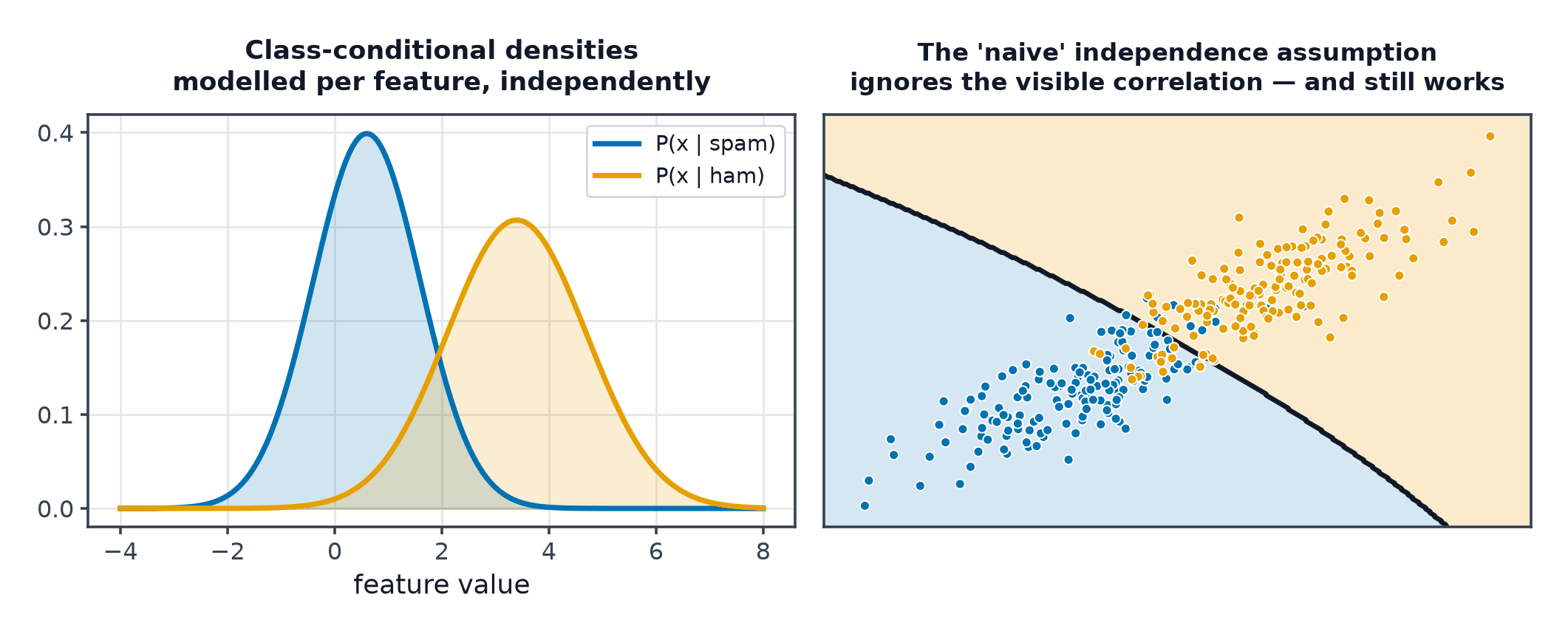
Naive Bayes assumes something that is almost never true — that every feature is independent given the class — and yet remains a strong baseline for text classification decades after more sophisticated methods appeared. Understanding why a false assumption still produces a useful classifier is the real lesson of this page.

Key idea

Assuming conditional independence of features makes the posterior trivial to compute — the probabilities are badly calibrated but the argmax is often right.

Naive Bayes models each feature's class-conditional density independently. The right panel shows it working on visibly correlated data — the probability estimates are badly calibrated, but the arg-max, and therefore the classification, often survives.

Bayes' rule applied to classification

$$p(y \mid x) = \frac{p(x \mid y)\,p(y)}{p(x)} \;\propto\; p(x \mid y)\,p(y)$$

Since $p(x)$ doesn't depend on $y$, classification reduces to comparing $p(x \mid y)\,p(y)$ across classes and picking the largest.

The naive independence assumption

Computing $p(x \mid y)$ directly for a feature vector $x = (x_1, \ldots, x_d)$ requires modelling the full joint distribution of all $d$ features given the class — infeasible with limited data. Naive Bayes assumes features are conditionally independent given the class:

$$p(x \mid y) = \prod_{i=1}^d p(x_i \mid y)$$

This turns an intractable joint estimation problem into $d$ separate, trivial 1-D estimation problems — the entire reason the method is fast and works with little data.

Variants by data type

• Gaussian NB: continuous features, each assumed Gaussian given the class.
• Multinomial NB: count data (word frequencies) — the standard choice for text classification.
• Bernoulli NB: binary features (word present/absent, ignoring count).

Laplace smoothing

A feature value never seen with a given class in training would give $p(x_i \mid y) = 0$, which zeroes out the entire product regardless of how strong the evidence from other features is. Laplace (add-one) smoothing adds a small pseudo-count to every possible value:

$$\hat p(x_i \mid y) = \frac{\text{count}(x_i, y) + \alpha}{\text{count}(y) + \alpha \cdot |\text{vocab}|}$$

Symbol	Meaning
$\alpha$	smoothing strength (typically 1)
$\lvert\text{vocab}\rvert$	number of distinct feature values

Working in log space

Multiplying many small probabilities underflows to zero in floating point. Naive Bayes is always implemented as a sum of log-probabilities instead:

$$\log p(y \mid x) \propto \log p(y) + \sum_i \log p(x_i \mid y)$$

Why it survives in text classification

Text features (word counts) are extremely high-dimensional and sparse, exactly the regime where naive Bayes's cheap per-feature estimation shines and where more data-hungry methods struggle without careful regularisation. Even though word co-occurrence obviously violates independence (words are correlated), the argmax decision often survives the miscalibration because the relative ranking of classes tends to be preserved even when the absolute probabilities are wrong.

Poor calibration, good ranking

Naive Bayes systematically produces overconfident probabilities (near 0 or 1) because the independence assumption double-counts correlated evidence — if two features are actually correlated, the model treats their combined evidence as if it came from two independent sources, inflating the posterior. The class ranking (and therefore accuracy) is often still correct even when the probability values themselves are not trustworthy.

Limitations

Beyond miscalibration: it cannot capture feature interactions (a combination of two words meaning something different from either alone), and it degrades on data where the independence assumption is violated in a way that actually flips the decision, not just the confidence.

Code: multinomial NB from scratch in log space, calibration check

naive_bayes_demo.py

import numpy as np
from sklearn.feature_extraction.text import CountVectorizer
from sklearn.naive_bayes import MultinomialNB

docs = [
    "great movie loved it", "terrible awful waste of time",
    "amazing acting great story", "boring terrible plot",
    "loved the amazing visuals", "awful boring waste",
]
labels = np.array([1, 0, 1, 0, 1, 0])  # 1 = positive, 0 = negative

vectorizer = CountVectorizer()
X = vectorizer.fit_transform(docs).toarray()

def fit_multinomial_nb(X, y, alpha=1.0):
    classes = np.unique(y)
    log_priors, feature_log_probs = {}, {}
    for c in classes:
        X_c = X[y == c]
        log_priors[c] = np.log(len(X_c) / len(X))
        word_counts = X_c.sum(axis=0) + alpha
        feature_log_probs[c] = np.log(word_counts / word_counts.sum())
    return log_priors, feature_log_probs

def predict_log_proba(X, log_priors, feature_log_probs):
    scores = np.array([
        [log_priors[c] + (x * feature_log_probs[c]).sum() for c in log_priors]
        for x in X
    ])
    return scores

log_priors, feature_log_probs = fit_multinomial_nb(X, labels)
scores = predict_log_proba(X, log_priors, feature_log_probs)
preds = scores.argmax(axis=1)
print("from-scratch predictions:", preds)

sk_model = MultinomialNB().fit(X, labels)
print("sklearn predictions:     ", sk_model.predict(X))
print("sklearn probabilities (often overconfident, near 0/1):")
print(sk_model.predict_proba(X).round(3))

The sklearn probabilities are typically pushed very close to 0 or 1 even on the training set — direct evidence of the overconfidence the independence assumption produces, even where the predicted labels themselves are correct.

When to reach for this

Data size	works even with very little data
Feature count	high-dimensional, sparse (text is the classic case)
Interpretability	moderate (per-feature log-probabilities are inspectable)
Training cost	extremely low — closed-form counting
Inference cost	very low — a sum of log-probabilities

See also

• Probability and Distributions — Bayes' rule and independence, derived in full.
• Text Preprocessing and Tokenization — producing the word-count features this model consumes.