PCA and SVD

Principal component analysis answers a simple question with surprisingly deep machinery: which few directions in a high-dimensional dataset capture most of what's actually going on? The answer — rotate onto the axes of greatest variance — turns out to be one of the most reused mathematical results in all of machine learning.

Key idea

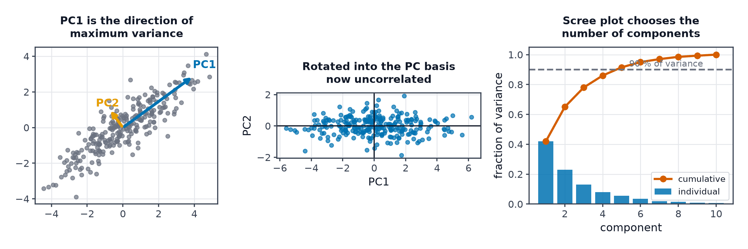
PCA rotates the data onto the axes of greatest variance; keeping the first few axes keeps most of the information.

PC1 is the direction of maximum variance and PC2 is orthogonal to it. Rotating into that basis leaves the data uncorrelated; the scree plot then tells you how many components you can keep before losing real signal.

The intuition: variance = information

A feature that never varies tells you nothing about which example you're looking at; a feature with large spread distinguishes examples strongly. PCA's core bet is that directions of high variance are the directions carrying the most information — not always true, but true often enough to be extremely useful.

Centring and scaling

Centring (subtracting the mean) is mandatory — PCA is defined in terms of variance around the mean, and skipping this step conflates "distance from zero" with "variance." Scaling (standardising each feature) is usually needed too, for the same reason as every other distance-based method in this section: a feature with a large numeric range will dominate the variance calculation regardless of its actual informativeness.

The covariance-matrix eigen route

Compute the covariance matrix $C = \frac{1}{n}X^\top X$ (assuming $X$ is already centred); its eigenvectors are the principal components, and its eigenvalues are the variance captured along each. The eigenvector with the largest eigenvalue is the direction of greatest variance — the first principal component.

The SVD route, and why implementations use it

Any centred matrix factors as $X = U\Sigma V^\top$ (from Linear Algebra). The columns of $V$ are exactly the principal components, and the squared singular values ($\Sigma^2$, divided by $n$) are exactly the eigenvalues of the covariance matrix. Real implementations use SVD directly on $X$ rather than explicitly forming $X^\top X$ first — computing $X^\top X$ squares the matrix's condition number, amplifying numerical error, which SVD avoids.

Explained variance ratio

$$\text{explained variance ratio of component } k = \frac{\lambda_k}{\sum_j \lambda_j}$$

The fraction of total variance captured by keeping component $k$; summing across the first $m$ components gives the cumulative variance retained by reducing to $m$ dimensions — the standard basis for choosing how many components to keep.

Symbol	Meaning
$C$	covariance matrix
$\lambda_k$	eigenvalue of the $k$-th principal component (its variance)
$U, \Sigma, V$	the SVD factorisation of $X$

Reconstruction and reconstruction error

Projecting onto $m < d$ components and projecting back approximates the original data; the reconstruction error (mean squared distance between original and reconstructed points) decreases monotonically as $m$ grows, reaching zero at $m = d$.

Loadings and interpreting components

Each principal component is a linear combination of the original features; the coefficients (loadings) show which original features contribute most to that component. Interpretation is genuinely limited, though: a component is a direction of variance, not necessarily a meaningful real-world concept, and loadings can mix many features in ways that resist a clean verbal description.

PCA whitening

Beyond just rotating and truncating, whitening additionally rescales each retained component to unit variance — producing features that are both decorrelated and equally scaled, sometimes useful as a preprocessing step for models sensitive to feature scale and correlation.

PCA is linear: what it cannot capture

PCA can only find linear combinations of features that capture variance — a dataset that lies on a curved (non-linear) manifold in the original space will not be well-approximated by any linear projection, no matter how many components are kept. Manifold Learning exists specifically for that case.

Kernel PCA

Applying the Kernel Methods trick to PCA lets it capture non-linear structure the same way kernel SVM captures non-linear decision boundaries — computing principal components in an implicit, higher-dimensional feature space.

Three distinct uses

Compression: reduce storage/compute by keeping only the components that matter. Visualisation: project to 2–3 dimensions for plotting (though see Manifold Learning for cases where PCA's linearity is too limiting). Decorrelation: PCA's components are, by construction, uncorrelated — useful as a preprocessing step before models that assume independent features.

Code: PCA via eigen decomposition and SVD, digit reconstructions

pca_svd_demo.py

import numpy as np
import matplotlib.pyplot as plt
from sklearn.decomposition import PCA
from sklearn.datasets import load_digits

rng = np.random.default_rng(0)
X = rng.normal(size=(200, 5)) @ rng.normal(size=(5, 5))  # correlated synthetic data
X_centered = X - X.mean(axis=0)

# --- Eigen decomposition route ---
cov = (X_centered.T @ X_centered) / len(X)
eigvals, eigvecs = np.linalg.eigh(cov)
order = np.argsort(eigvals)[::-1]
eigvals, eigvecs = eigvals[order], eigvecs[:, order]

# --- SVD route ---
U, S, Vt = np.linalg.svd(X_centered, full_matrices=False)
svd_eigvals = (S ** 2) / len(X)

print("eigen-decomposition eigenvalues:", np.round(eigvals, 4))
print("SVD-derived eigenvalues:        ", np.round(svd_eigvals, 4), "  <- should match")

# --- sklearn PCA on real data: digits ---
digits = load_digits()
X_digits = digits.data
pca = PCA(n_components=50).fit(X_digits)
cumvar = np.cumsum(pca.explained_variance_ratio_)
print(f"\ncomponents needed for 90% variance: {np.argmax(cumvar >= 0.9) + 1}")

fig, axes = plt.subplots(1, 4, figsize=(12, 3))
axes[0].imshow(X_digits[0].reshape(8, 8), cmap="gray"); axes[0].set_title("original")
for ax, n_comp in zip(axes[1:], [5, 20, 50]):
    pca_n = PCA(n_components=n_comp).fit(X_digits)
    reconstructed = pca_n.inverse_transform(pca_n.transform(X_digits[:1]))
    ax.imshow(reconstructed.reshape(8, 8), cmap="gray")
    ax.set_title(f"{n_comp} components")
plt.savefig("pca_reconstruction.png")

When to reach for this

Data size	scales well
Feature count	designed for high-dimensional data
Interpretability	moderate (loadings), lower for later components
Training cost	$O(nd^2)$ or $O(d^3)$ depending on route
Inference cost	one matrix multiplication to project a new point

See also

• Linear Algebra — the eigenvector/SVD machinery this method is built on.
• Manifold Learning — non-linear dimensionality reduction for data PCA cannot flatten correctly.