Random Forests and Bagging

A single unconstrained decision tree overfits badly. Grow a few hundred of them, each on a slightly different random sample of the data, and average their predictions — and the overfitting largely cancels out. That's the entire idea behind bagging, and random forests are bagging applied specifically to trees with one extra trick.

Key idea

Bagging cuts variance by averaging decorrelated models; random feature subsets are what make the trees decorrelated enough for it to work.

Averaging many high-variance trees, each fitted to a bootstrap sample, cancels their individual errors. The forest's boundary is smooth even though every tree composing it is a staircase.

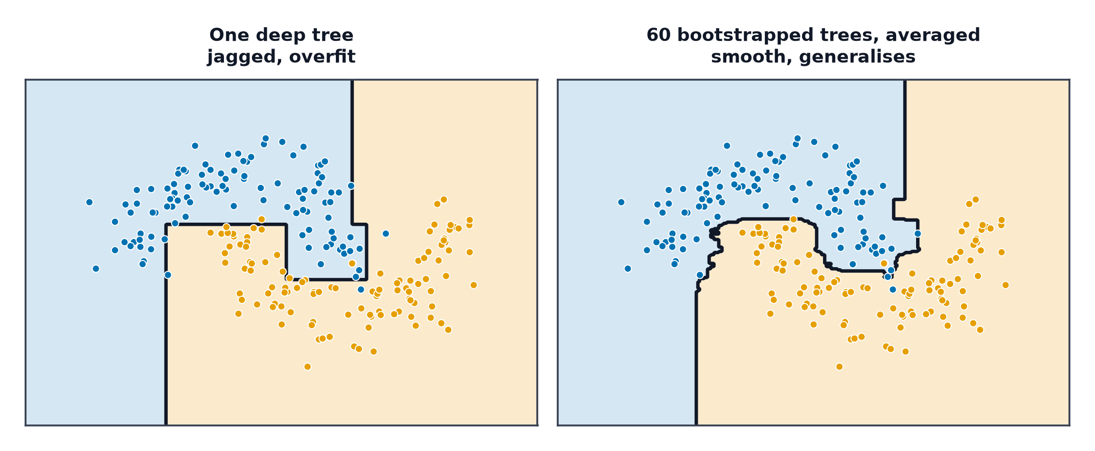
Bootstrap sampling

For each of $B$ trees, draw a bootstrap sample: $n$ examples sampled with replacement from the original $n$-example training set. Roughly 63% of the original examples appear at least once in each bootstrap sample; the rest are duplicated or omitted at random.

Bagging as variance reduction, with the maths

For $B$ predictors each with variance $\sigma^2$ and pairwise correlation $\rho$, the variance of their average is:

$$\text{Var}\left(\frac{1}{B}\sum_b \hat f_b\right) = \rho\sigma^2 + \frac{(1-\rho)\sigma^2}{B}$$

Symbol	Meaning
$B$	number of trees in the ensemble
$\sigma^2$	variance of a single tree's prediction
$\rho$	correlation between any pair of trees' predictions

As $B \to \infty$, the second term vanishes — but the first term, $\rho\sigma^2$, remains regardless of how many trees you add. This is why decorrelating the trees matters more than simply adding more of them: averaging highly correlated trees barely reduces variance beyond a certain point, since $\rho\sigma^2$ is the floor.

Random feature subsets at each split

Bootstrap sampling alone doesn't decorrelate trees much, because a single very strong feature will dominate the root split of nearly every tree regardless of which bootstrap sample it saw. Random forests add a second randomisation: at each split, only a random subset of features (typically $\sqrt{d}$ for classification) is considered. This forces different trees to rely on different features, directly lowering $\rho$ in the variance formula above.

Out-of-bag error as free validation

Since each tree's bootstrap sample omits roughly 37% of the training examples, those omitted ("out-of-bag") examples can be used to validate that specific tree — averaging out-of-bag predictions across all trees gives an honest performance estimate without needing a separate held-out validation set.

Hyperparameters that matter

• n_estimators (number of trees): more is (almost) always better, with diminishing returns; rarely overfits by itself.
• max_features (features considered per split): the main decorrelation knob.
• max_depth, min_samples_leaf: control individual tree complexity, and therefore $\sigma^2$.

Permutation importance vs. impurity importance

Impurity-based importance (from Decision Trees) is biased toward high-cardinality features. Permutation importance instead measures how much validation performance drops when a single feature's values are randomly shuffled — a direct, model-agnostic causal test rather than an internal training-time bookkeeping statistic, and it is not biased toward high-cardinality noise features.

Extremely randomised trees

Extra Trees goes one step further: instead of searching for the best threshold at each candidate feature, it picks a random threshold. This trades a small amount of bias for further variance reduction and faster training.

Where random forests still beat gradient boosting

Random forests are far more robust to noisy labels and outliers (each tree only sees part of the data, so a mislabelled point has limited influence), parallelise trivially (every tree is independent), and need almost no hyperparameter tuning to get a reasonable result — Gradient Boosting usually wins on raw accuracy with careful tuning, but random forests remain the better default when tuning time is scarce or labels are noisy.

Code: random forest vs. single tree, OOB score, importance bias

random_forest_demo.py

import numpy as np
from sklearn.ensemble import RandomForestClassifier
from sklearn.tree import DecisionTreeClassifier
from sklearn.inspection import permutation_importance
from sklearn.model_selection import train_test_split, cross_val_score

rng = np.random.default_rng(0)
n = 500
X_informative = rng.normal(size=(n, 3))
X_nuisance_high_card = rng.integers(0, 1000, size=(n, 1))  # high-cardinality, uninformative
X = np.hstack([X_informative, X_nuisance_high_card])
y = (X_informative[:, 0] + X_informative[:, 1] > 0).astype(int)

X_train, X_test, y_train, y_test = train_test_split(X, y, test_size=0.3, random_state=0)

tree = DecisionTreeClassifier(random_state=0).fit(X_train, y_train)
forest = RandomForestClassifier(n_estimators=200, oob_score=True, random_state=0).fit(X_train, y_train)

print(f"single tree test accuracy:  {tree.score(X_test, y_test):.3f}")
print(f"random forest test accuracy: {forest.score(X_test, y_test):.3f}")
print(f"random forest OOB score:     {forest.oob_score_:.3f}  (should track test accuracy closely)")

# --- Importance bias: the nuisance column is uninformative but high-cardinality ---
print("\nimpurity-based importance (biased toward high-cardinality noise):")
print(forest.feature_importances_)

perm = permutation_importance(forest, X_test, y_test, n_repeats=10, random_state=0)
print("permutation importance (correctly near-zero for the noise column):")
print(perm.importances_mean)

The nuisance column (index 3, high-cardinality but uninformative) typically shows a non-trivial impurity-based importance despite contributing nothing to the true label — permutation importance should correctly rank it near zero.

When to reach for this

Data size	small to large
Feature count	handles many features well, including irrelevant ones
Interpretability	moderate (feature importance, but not a single readable path)
Training cost	moderate, parallelises trivially across trees
Inference cost	proportional to number of trees

See also

• Decision Trees — the base learner this method ensembles.
• Gradient Boosting — the sequential alternative to this parallel ensembling approach.