Regularization: Ridge, Lasso, Elastic Net

Unregularised least squares fits every quirk of the training sample, including its noise, once you have enough features relative to examples. Ridge, lasso, and elastic net apply the general regularisation principle from Overfitting and Regularization specifically to linear models, each trading a little bias for a large drop in variance.

Key idea

Penalising coefficient size trades a little bias for a large drop in variance, and the shape of the penalty decides whether coefficients shrink or vanish.

Why unregularised least squares overfits with many features

With $d$ features and $n \approx d$ examples, the normal equation can perfectly fit the training data (zero residual) by exploiting noise — the fitted line contorts to match every random fluctuation, and predictions on new data are unstable and poor.

Ridge (L2): closed form

$$w^*_{\text{ridge}} = (X^\top X + \lambda I)^{-1}X^\top y$$

Adding $\lambda I$ to $X^\top X$ before inverting guarantees the matrix is invertible even when $X^\top X$ alone is singular (the multicollinearity case from Linear Regression) — geometrically, ridge shrinks every coefficient toward zero in proportion to how much it contributes to overfitting, but never sets one to exactly zero.

Lasso (L1) and why the corner causes sparsity

The corner is the whole mechanism. Because the L1 region's vertices lie on the axes, the first point of contact with the loss contour is very often one of them — and at that point a coefficient is exactly zero.

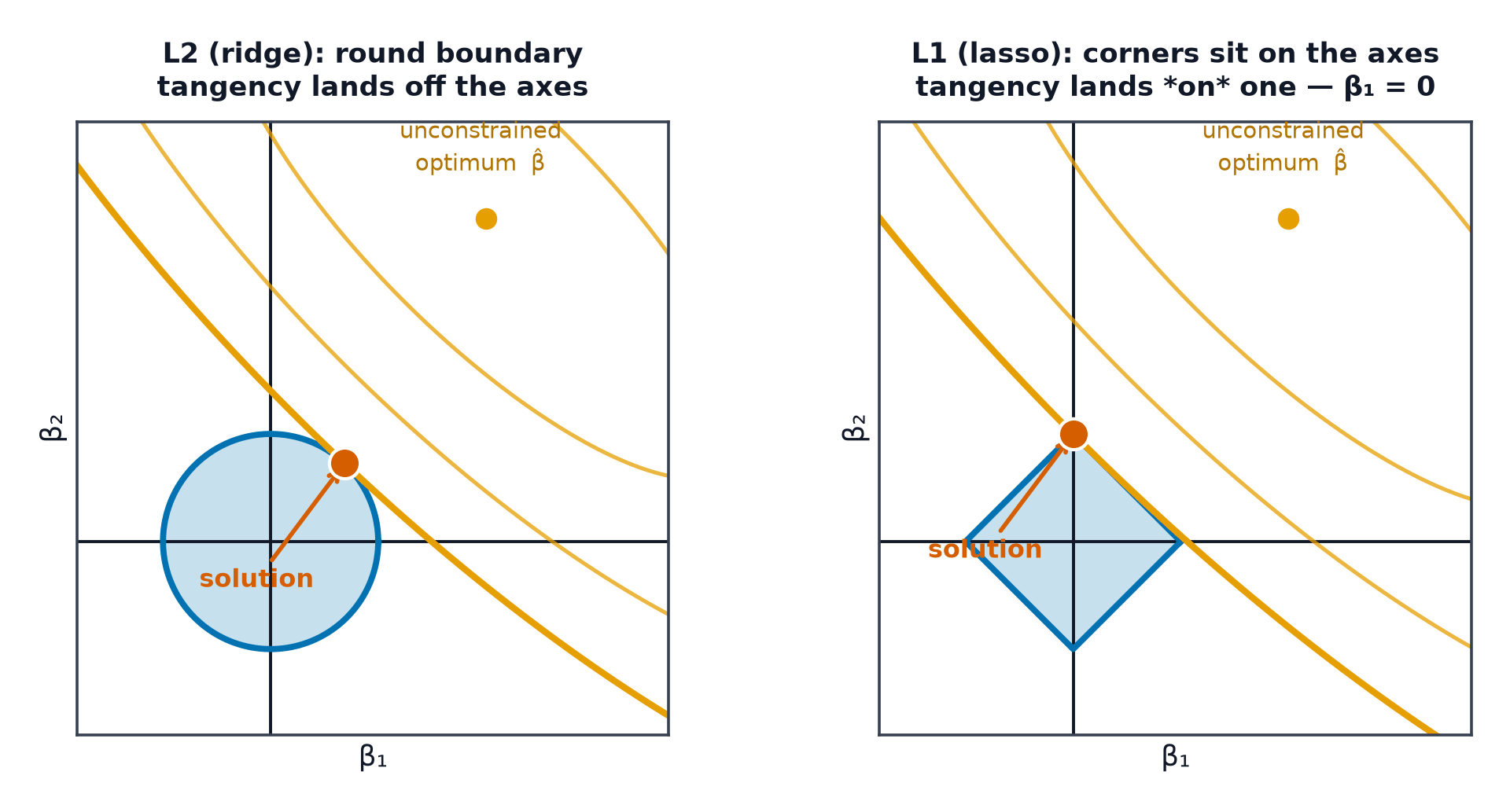
Lasso minimises $\|Xw - y\|_2^2 + \lambda\|w\|_1$, with no closed form (solved by coordinate descent or similar iterative methods). The geometric argument: constrained optimisation of a smooth loss against an L1 ball (a diamond in 2D) tends to land at a corner of the diamond, where one or more coordinates are exactly zero — against an L2 ball (a circle), the smooth loss contours are tangent to the circle at an arbitrary point, essentially never exactly on an axis.

Symbol	Meaning
$\lambda$	regularisation strength
$I$	identity matrix
$\|w\|_1, \|w\|_2$	L1 and L2 norms of the weight vector

Elastic net

$$L(w) = \|Xw - y\|_2^2 + \lambda\big(\alpha\|w\|_1 + (1-\alpha)\|w\|_2^2\big)$$

Combines both penalties, controlled by mixing parameter $\alpha$ — useful when features are both numerous and correlated, since pure lasso tends to arbitrarily pick one of a correlated group and zero out the rest, while the L2 component stabilises that selection.

Choosing λ by cross-validation

$\lambda$ is a hyperparameter, not learned by the training objective itself — sweep a range of values and pick the one minimising validation error (Train/Validation/Test Splits), never the one minimising training error (which is always $\lambda = 0$).

Standardisation is mandatory

The penalty term treats every coefficient's scale identically, so a feature measured in thousands (income) will be penalised far more harshly than one measured in single digits (age) unless both are standardised first — otherwise the regularisation strength isn't actually comparable across features.

Coefficient paths

Both penalties shrink coefficients as α rises, but only lasso sets them to exactly zero — and it does so one at a time, which is what makes it a feature selector. Ridge keeps every coefficient, however small.

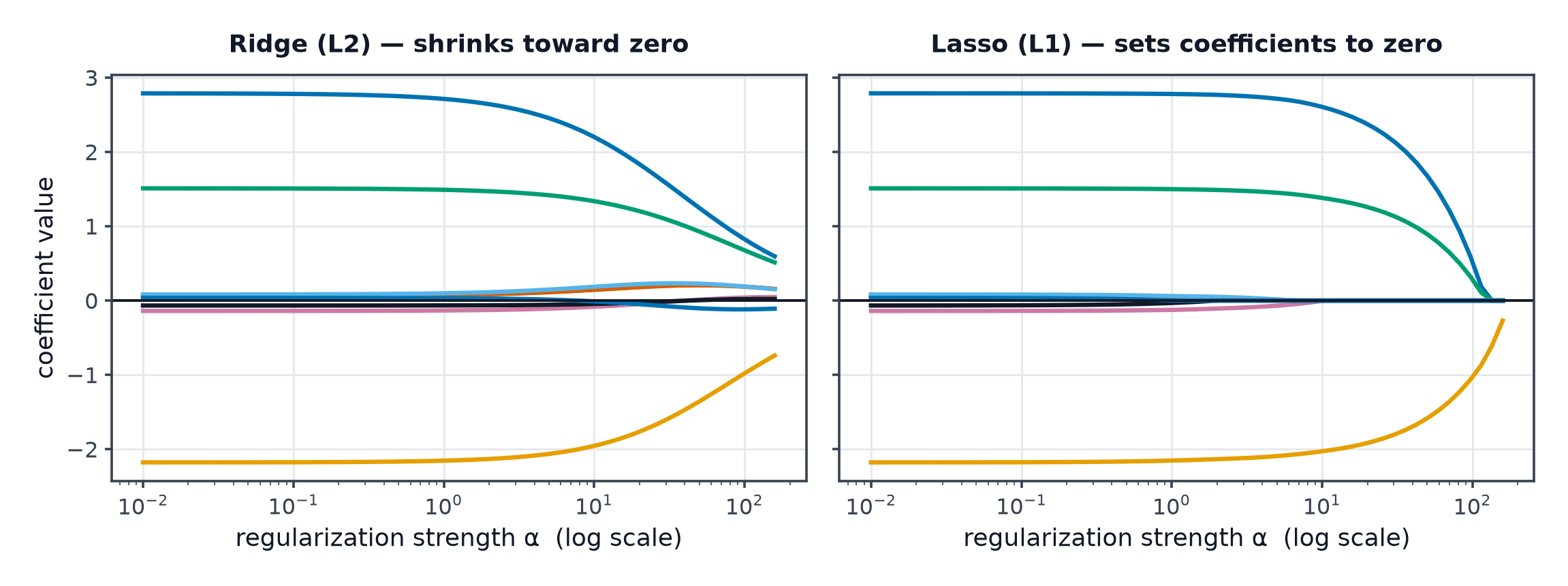
Plotting each coefficient's value as $\lambda$ sweeps from 0 to large reveals ridge's smooth shrinkage toward (but not to) zero, versus lasso's coefficients hitting exactly zero one by one as $\lambda$ grows — a direct visual confirmation of the sparsity argument above.

Lasso as feature selection, and its instability

Because lasso zeros out coefficients, it performs automatic feature selection. The caveat: with correlated features, small changes in the data can cause lasso to select a different subset of the correlated group each time — the selection is not stable, even though predictive performance is.

Selection table

Situation	Reach for
Many correlated features, want stable predictions	Ridge
Want automatic feature selection, features roughly independent	Lasso
Many features, some correlated groups	Elastic net

Code: RidgeCV/LassoCV coefficient paths

ridge_lasso_paths_demo.py

import numpy as np
from sklearn.linear_model import RidgeCV, LassoCV
from sklearn.preprocessing import StandardScaler

rng = np.random.default_rng(0)
n, d = 100, 20
X = rng.normal(size=(n, d))
true_w = np.zeros(d)
true_w[:3] = [3.0, -2.0, 1.5]  # only 3 of 20 features matter
y = X @ true_w + rng.normal(scale=0.5, size=n)
X_scaled = StandardScaler().fit_transform(X)

alphas = np.logspace(-3, 2, 30)
ridge = RidgeCV(alphas=alphas).fit(X_scaled, y)
lasso = LassoCV(alphas=alphas, max_iter=5000).fit(X_scaled, y)

print(f"ridge best alpha: {ridge.alpha_:.4f}, nonzero-ish coefs (>0.01): {np.sum(np.abs(ridge.coef_) > 0.01)}")
print(f"lasso best alpha: {lasso.alpha_:.4f}, exact-zero coefs: {np.sum(lasso.coef_ == 0.0)} of {d}")
print("lasso selected features (nonzero):", np.nonzero(lasso.coef_)[0])
print("  (true nonzero features were: [0, 1, 2])")

Lasso's selected features should closely match the three that actually matter, while ridge keeps all 20 coefficients nonzero but shrinks the 17 irrelevant ones toward (not to) zero.

When to reach for this

Data size	works well down to small $n$ relative to $d$
Feature count	designed for high-dimensional settings
Interpretability	ridge: moderate; lasso: high (sparse)
Training cost	ridge: one matrix inversion; lasso: iterative, slightly more
Inference cost	same as linear regression — one dot product

See also

• Overfitting and Regularization — the general theory these three methods instantiate.
• Linear Regression — the unregularised baseline these methods stabilise.