Support Vector Machines

Logistic regression finds a separating line. Support vector machines find the separating line furthest from every training point — and it turns out only a handful of points (the "support vectors") actually determine where that line goes. The rest of the training set could be deleted without changing the model at all.

Key idea

Only the support vectors matter — the rest of the training set could be deleted without changing the model.

The maximum-margin idea

The separator is placed to maximise the distance to the nearest point of either class. Only the three circled points — the support vectors, which sit exactly on the margin — determine it; deleting any other point changes nothing.

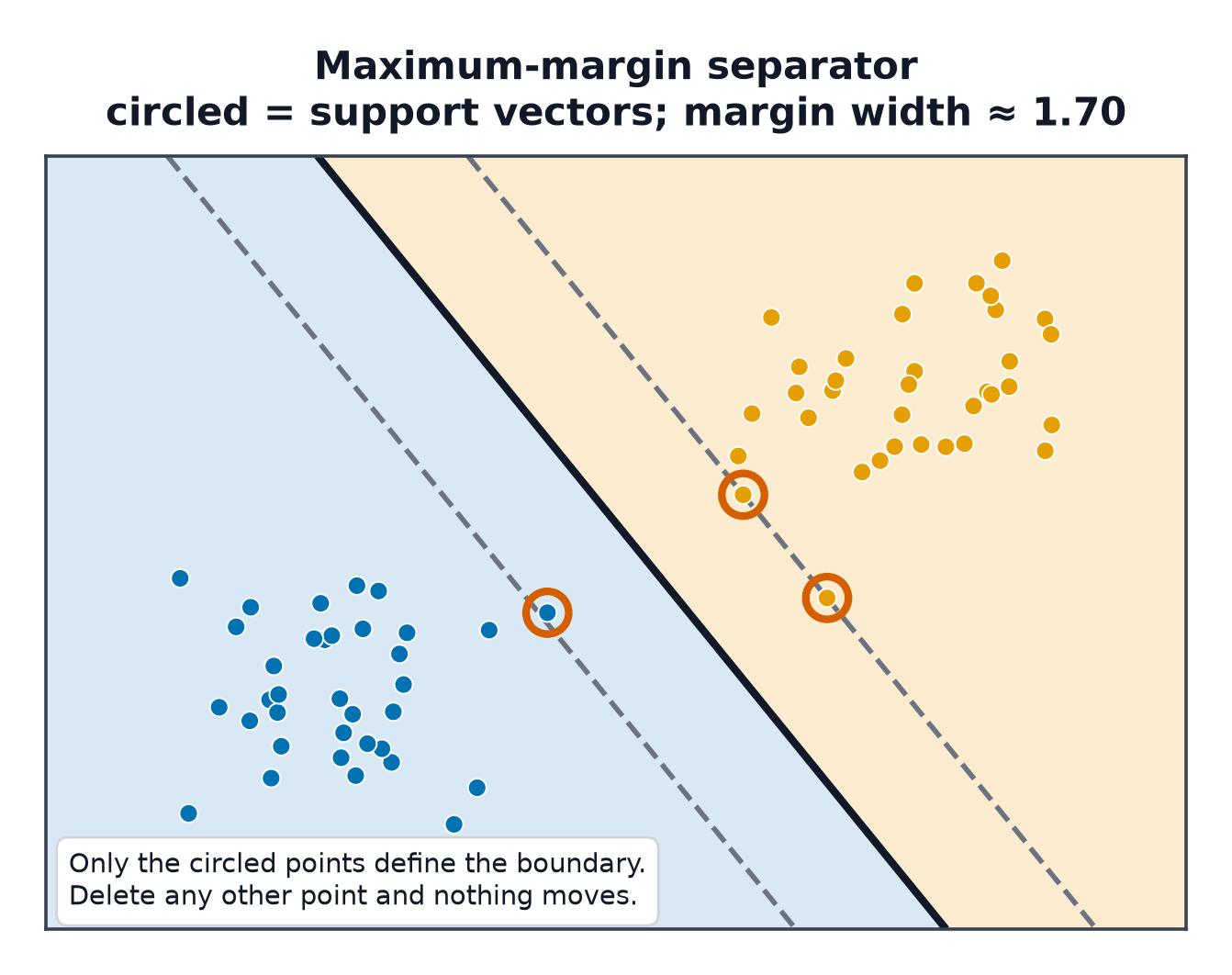
Among the infinitely many lines that separate two classes, SVM picks the one maximising the distance to the nearest point of either class — intuitively, the line with the most "breathing room," which tends to generalise better to new points near the boundary.

Functional vs. geometric margin

The functional margin $y_i(w^\top x_i + b)$ scales with $\|w\|$; the geometric margin $\frac{y_i(w^\top x_i + b)}{\|w\|}$ is scale-invariant — the actual perpendicular distance from the point to the boundary, which is what SVM actually maximises.

The hard-margin primal

$$\min_{w,b} \frac{1}{2}\|w\|^2 \quad \text{s.t.} \quad y_i(w^\top x_i + b) \ge 1 \; \forall i$$

Minimising $\|w\|^2$ is equivalent to maximising the margin $\frac{2}{\|w\|}$; the constraint requires every point correctly classified with at least unit functional margin. This only has a solution when the classes are perfectly separable.

The soft margin and C

Real data is rarely perfectly separable. The soft-margin formulation introduces slack variables $\xi_i \ge 0$ allowing some points to violate the margin (or even be misclassified), penalised by a cost $C$:

$$\min_{w,b,\xi} \frac{1}{2}\|w\|^2 + C\sum_i \xi_i \quad \text{s.t.} \quad y_i(w^\top x_i + b) \ge 1 - \xi_i, \; \xi_i \ge 0$$

Hinge loss as the unconstrained view

The soft-margin problem is equivalent to minimising hinge loss (from Loss Functions) plus an L2 penalty:

$$\min_{w,b} \frac{1}{2}\|w\|^2 + C\sum_i \max(0, 1 - y_i(w^\top x_i + b))$$

Symbol	Meaning
$w, b$	the separating hyperplane's normal vector and offset
$\xi_i$	slack allowing point $i$ to violate the margin
$C$	cost of margin violations — the bias/variance dial
$\alpha_i$	the dual's Lagrange multipliers, one per training point

The dual formulation

Lagrangian duality rewrites the problem entirely in terms of dot products between training points and a set of multipliers $\alpha_i \ge 0$ (one per point). This matters because: (1) points with $\alpha_i = 0$ never influence the boundary at all — only points with $\alpha_i > 0$ (the support vectors) do; (2) the dual depends on data only through pairwise dot products, which is exactly the opening Kernel Methods needs to swap in a kernel and get a non-linear boundary for free.

Support vectors

Points lying exactly on the margin, or violating it, are support vectors — everything else can be deleted from the training set post-training with zero effect on predictions.

SVM for regression (SVR)

The same margin idea flipped: instead of separating classes, fit a function such that most points fall within an $\epsilon$-tube around it, penalising only points outside that tube.

Scaling requirements

Like kNN, SVM's distance-based geometry requires standardised features — an unscaled feature with a large numeric range will dominate the margin computation.

C as the bias/variance dial

Large $C$ penalises margin violations heavily — a narrow margin that fits training data tightly (low bias, high variance, risk of overfitting). Small $C$ tolerates more violations for a wider margin (higher bias, lower variance).

Code: LinearSVC, margins plotted, a C sweep

svm_demo.py

import numpy as np
import matplotlib.pyplot as plt
from sklearn.svm import LinearSVC
from sklearn.datasets import make_blobs

X, y = make_blobs(n_samples=100, centers=2, cluster_std=1.2, random_state=6)

fig, axes = plt.subplots(1, 3, figsize=(15, 4))
for ax, C in zip(axes, [0.01, 1, 100]):
    model = LinearSVC(C=C, max_iter=10000).fit(X, y)
    w, b = model.coef_[0], model.intercept_[0]

    xx = np.linspace(X[:, 0].min(), X[:, 0].max(), 100)
    yy = -(w[0] * xx + b) / w[1]
    margin = 1 / np.linalg.norm(w)
    yy_up = yy + margin * np.sqrt(1 + (w[0]/w[1])**2)
    yy_down = yy - margin * np.sqrt(1 + (w[0]/w[1])**2)

    ax.scatter(X[:, 0], X[:, 1], c=y, edgecolors="k")
    ax.plot(xx, yy, "k-")
    ax.plot(xx, yy_up, "k--"); ax.plot(xx, yy_down, "k--")
    ax.set_title(f"C={C}, margin width={2*margin:.2f}")
plt.savefig("svm_margins.png")

As $C$ grows from 0.01 to 100, the plotted margin width should visibly shrink — the model tightens its boundary around the training points instead of maximising breathing room.

When to reach for this

Data size	small-to-medium (kernel SVMs scale poorly past tens of thousands of points)
Feature count	works well even when $d > n$
Interpretability	linear SVM: moderate; kernel SVM: low
Training cost	quadratic-to-cubic in $n$ for kernel SVMs
Inference cost	proportional to number of support vectors

See also

• Kernel Methods — extending this to non-linear boundaries via the dual's dot-product structure.
• Loss Functions — hinge loss, the unconstrained equivalent of the soft margin.