CNN Architectures

Fifteen years of vision architecture research boiled down to a handful of ideas that survived contact with reality: go deeper, but only once you can actually train the depth; use small filters repeatedly rather than large ones once; and share computation aggressively when compute or memory is scarce. Nearly every architecture below is one of these ideas, applied and refined.

Key idea

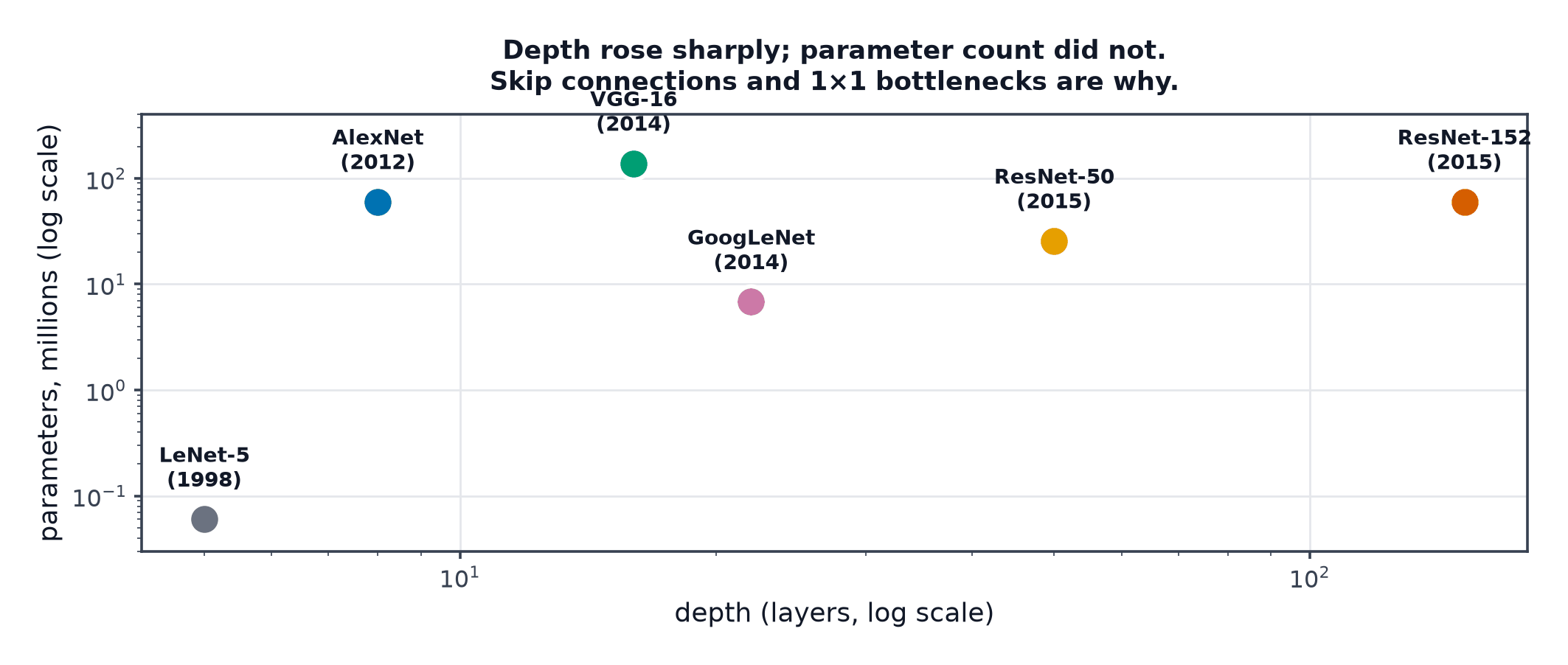
Architectures evolved by making networks deeper while finding ways to keep them trainable and affordable.

Depth grew by more than an order of magnitude while parameter counts did not — VGG-16 has more parameters than ResNet-152. Skip connections and 1×1 bottlenecks are what decoupled the two.

LeNet-5

One of the earliest practical CNNs (1998), designed for handwritten digit recognition — a small stack of convolution and pooling layers followed by fully-connected layers, establishing the basic conv-pool-conv-pool-FC pattern that every later architecture, in some form, still follows.

AlexNet, and what 2012 actually changed

AlexNet's 2012 ImageNet win is widely credited with kickstarting the deep learning era, but the architectural ideas were mostly already known — what actually changed was the combination: ReLU (Activation Functions) instead of saturating sigmoid/tanh, dropout (Regularization in Deep Nets) as regularisation, GPUs making a network of this scale computationally feasible to train at all, and a dataset (ImageNet) large enough to justify that scale.

VGG and the 3×3 stacking argument

VGG's key insight: two stacked $3\times3$ convolutions have the same receptive field as one $5\times5$ convolution, but with fewer total parameters ($2 \times 3^2 = 18$ vs. $5^2 = 25$ per channel pair) and an extra non-linearity in between — stacking small filters is both cheaper and more expressive than using larger filters directly, an argument that shaped nearly every architecture that followed.

Inception and multi-scale blocks

Rather than committing to a single filter size per layer, an Inception block runs several filter sizes ($1\times1$, $3\times3$, $5\times5$) in parallel on the same input and concatenates their outputs — captures features at multiple spatial scales simultaneously, at the cost of a more complex, harder-to-tune block design.

ResNet, and why skip connections mattered most here

Skip Connections and Depth covers the general mechanism in full; in the CNN context specifically, residual connections were what finally let networks scale past roughly 20 layers without the degradation problem — ResNet variants reaching over 100 layers became not just trainable but state-of-the-art, directly because of this fix.

DenseNet

Connects every layer directly to every subsequent layer within a block (not just the immediately preceding one, as in a standard residual connection) — maximises gradient flow and feature reuse throughout the network, at the cost of substantially higher memory usage from retaining every intermediate feature map for these dense connections.

MobileNet and depthwise separable convolutions

Built specifically for resource-constrained (mobile, edge) deployment, using The Convolution Operation's depthwise separable convolutions throughout to cut parameters and compute by roughly an order of magnitude relative to standard convolutions, at a modest accuracy cost — the standard architecture family when inference must run on-device rather than on a server.

EfficientNet and compound scaling

Rather than scaling depth, width, or input resolution independently (the ad-hoc approach most earlier architectures took when creating "small/medium/large" variants), EfficientNet scales all three jointly, according to a fixed ratio found via a systematic search — produces a family of models along a smoother, more efficient accuracy/compute trade-off curve than independently-scaled variants achieve.

Family	Key innovation
LeNet-5	the basic conv-pool-FC pattern
AlexNet	ReLU + dropout + GPU scale, combined
VGG	small stacked filters beat large single filters
Inception	parallel multi-scale filters per block
ResNet	residual connections enable real depth
DenseNet	dense connections maximise feature reuse
MobileNet	depthwise separable convolutions for efficiency
EfficientNet	joint depth/width/resolution scaling
ConvNeXt	convolutional design informed by transformer successes

ConvNeXt, and convolutions answering back to transformers

After Vision Transformers demonstrated strong results on image tasks, ConvNeXt revisited the standard ResNet design and modernised it with several transformer-inspired training and architectural choices (larger kernels, different normalisation placement, updated training recipes) while remaining a pure CNN — showing much of the transformer's apparent advantage came from modern training practices rather than the architecture itself being fundamentally superior for vision.

Comparison table

	Parameters	Relative FLOPs	Accuracy tier	Typical use
ResNet-50	~25M	moderate	strong baseline	general-purpose default
MobileNetV3	~5M	low	good for its size	mobile/edge deployment
EfficientNet-B0	~5M	low	strong for its size	efficiency-focused deployment
ConvNeXt	~28M+	moderate-high	very strong	when accuracy is the priority

How to choose: the honest default

Unless you have a specific reason not to (extreme resource constraints, a research need to compare against transformers), a pretrained ResNet or EfficientNet backbone remains a perfectly strong, well-understood, well-supported default choice for most practical vision tasks — see Transfer Learning for Vision for using one.

Code: three pretrained backbones compared

cnn_architectures_demo.py

import time
import torch
from torchvision import models, transforms
from PIL import Image
import numpy as np

# --- The running image, standing in as a synthetic array ---
rng = np.random.default_rng(0)
img_array = rng.integers(0, 256, size=(224, 224, 3), dtype=np.uint8)
img = Image.fromarray(img_array, mode="RGB")

transform = transforms.Compose([
    transforms.Resize((224, 224)), transforms.ToTensor(),
    transforms.Normalize(mean=[0.485, 0.456, 0.406], std=[0.229, 0.224, 0.225]),
])
input_tensor = transform(img).unsqueeze(0)

backbones = {
    "ResNet-50": models.resnet50(weights=models.ResNet50_Weights.DEFAULT),
    "MobileNetV3-Small": models.mobilenet_v3_small(weights=models.MobileNet_V3_Small_Weights.DEFAULT),
    "EfficientNet-B0": models.efficientnet_b0(weights=models.EfficientNet_B0_Weights.DEFAULT),
}

print(f"{'model':20s} | {'params':>10s} | {'inference time':>15s} | {'top prediction':>15s}")
for name, model in backbones.items():
    model.eval()
    n_params = sum(p.numel() for p in model.parameters())
    start = time.perf_counter()
    with torch.no_grad():
        output = model(input_tensor)
    elapsed = time.perf_counter() - start
    top_class = output.argmax(dim=1).item()
    print(f"{name:20s} | {n_params:10,d} | {elapsed*1000:13.2f}ms | class {top_class:9d}")

See also

• The Convolution Operation and Pooling and Shape Arithmetic — the two operations every architecture here is assembled from.
• Transfer Learning for Vision — using one of these pretrained backbones on a new task.