CNN Interpretability

A model that's 98% accurate on your test set can still be completely wrong about why. A famous, real example: a classifier trained to distinguish huskies from wolves turned out to be detecting snow in the background, not the animal — accurate on a test set that happened to reflect the same correlation, and silently broken the moment that correlation didn't hold. Interpretability tools exist to catch exactly this before deployment, not after.

Key idea

Attribution methods show where a prediction came from, which is how you catch a model that is right for the wrong reason.

Grad-CAM weights the final convolutional feature maps by the gradient of the target class, producing a coarse map of what the model actually used. It shows *where* the evidence was, not *why* it counted as evidence.

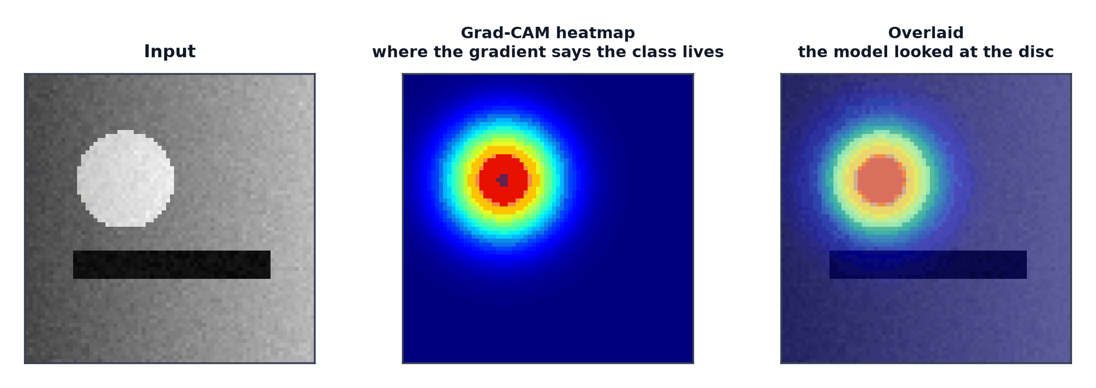
Why accuracy alone hides shortcut learning

A model optimises whatever correlates with the label in its training data — if a spurious feature (background snow, a watermark, an imaging artefact specific to one data source) happens to correlate with the label in that data, the model may learn to rely on the spurious feature instead of the genuine one, and accuracy alone cannot distinguish "learned the real pattern" from "learned a shortcut that happened to work on this test set."

Filter visualisation in the first layer

The very first convolutional layer's learned filters can be directly visualised as small images (they operate on raw pixel values, so their weights are interpretable as image patches) — a healthy, well-trained first layer typically shows edge and colour-blob detectors resembling classic hand-designed filters; a first layer that looks like unstructured noise suggests a training problem.

Feature maps per layer

Passing a real image through the network and visualising the resulting activation map at any given layer shows what that layer responds to for that specific image — early layers show simple edges/textures activating in a spatially recognisable pattern; deeper layers show increasingly abstract, less visually interpretable patterns.

Saliency maps via input gradients

Compute $\partial(\text{predicted class score})/\partial(\text{input pixels})$ — which input pixels, if changed slightly, would most change the prediction — and visualise this gradient directly as a heatmap over the input image. The main problem: raw input gradients tend to be visually noisy, without further processing, making them harder to interpret cleanly than the methods below.

Grad-CAM

Rather than gradients with respect to the raw input pixels, Grad-CAM uses gradients with respect to the last convolutional layer's feature maps — because that layer still has spatial structure (unlike the fully-connected layers after it) but has already built up substantial semantic abstraction (unlike the earlier layers), producing a heatmap that's both spatially meaningful and semantically relevant.

$$L_{\text{Grad-CAM}} = \text{ReLU}\left(\sum_k \alpha_k A^k\right), \qquad \alpha_k = \frac{1}{Z}\sum_{i,j} \frac{\partial y^c}{\partial A^k_{ij}}$$

Symbol	Meaning
$A^k$	the $k$-th feature map of the target convolutional layer
$\alpha_k$	the global-average-pooled gradient — how important feature map $k$ is to class $c$
$y^c$	the predicted score for target class $c$

The final ReLU keeps only positive influence (regions that increase the target class score), discarding regions that push the prediction toward other classes.

Grad-CAM++ and Score-CAM, briefly

Grad-CAM++ refines the weighting to better handle multiple instances of the same class within one image. Score-CAM replaces the gradient-based weighting entirely with a forward-pass-only approach (masking the input with each feature map and measuring the resulting score change directly) — avoids some gradient-based artefacts, at higher computational cost (many forward passes instead of one backward pass).

Occlusion sensitivity

The assumption-free baseline: systematically slide an occluding patch (e.g. a grey square) across the image, rerunning the model at each position, and record how much the target class's score drops when each region is occluded — directly measures each region's causal importance to the prediction, without relying on gradients at all, at the cost of many forward passes.

Integrated gradients

Rather than a single gradient at the actual input, integrate gradients along a path from a baseline (e.g. a black image) to the actual input — addresses a known weakness of raw input gradients (they can be near-zero even for genuinely important pixels, if the model's response has saturated at that specific input) by aggregating gradient information across the whole path instead of one point.

SHAP for images

Applies SHAP's game-theoretic attribution framework (fairly distributing a prediction's "credit" among input features, based on their marginal contribution across many possible feature subsets) to image regions — computationally expensive for images specifically, given the very large number of possible pixel-region subsets, but grounded in a more rigorous theoretical framework than most gradient-based methods.

The honest limits

Every method here produces a hypothesis about what the model is responding to — none is a certified, complete explanation of the model's internal computation. Attribution maps can be locally unstable (a visually imperceptible input change can shift the map substantially, without changing the prediction) and can disagree with each other on the same input — treat attribution as a diagnostic lead worth investigating, not a definitive verdict on model behaviour.

Using attribution during dataset debugging

Running Grad-CAM (or similar) across a sample of correctly-classified training or validation images, looking specifically for cases where the highlighted region is not the actual object of interest — background, a watermark, an artefact — is a direct, practical way to catch the husky/wolf-style shortcut-learning failure before it reaches production.

Code: Grad-CAM from scratch with hooks, occlusion sensitivity

cnn_interpretability_demo.py

import torch
import torch.nn.functional as F
from torchvision import models, transforms
from PIL import Image
import numpy as np
import matplotlib.pyplot as plt

model = models.resnet18(weights=models.ResNet18_Weights.DEFAULT)
model.eval()

rng = np.random.default_rng(0)
img_array = rng.integers(0, 256, size=(224, 224, 3), dtype=np.uint8)
img = Image.fromarray(img_array, mode="RGB")
transform = transforms.Compose([
    transforms.ToTensor(),
    transforms.Normalize(mean=[0.485, 0.456, 0.406], std=[0.229, 0.224, 0.225]),
])
input_tensor = transform(img).unsqueeze(0)

# --- Grad-CAM via hooks on the last conv layer ---
activations, gradients = {}, {}
def forward_hook(module, input, output): activations["value"] = output
def backward_hook(module, grad_input, grad_output): gradients["value"] = grad_output[0]

target_layer = model.layer4[-1]
target_layer.register_forward_hook(forward_hook)
target_layer.register_full_backward_hook(backward_hook)

output = model(input_tensor)
top_class = output.argmax(dim=1)
model.zero_grad()
output[0, top_class].backward()

pooled_gradients = gradients["value"].mean(dim=[0, 2, 3])
activation_maps = activations["value"][0]
for i in range(activation_maps.shape[0]):
    activation_maps[i] *= pooled_gradients[i]
heatmap = F.relu(activation_maps.mean(dim=0)).detach().numpy()
heatmap = heatmap / (heatmap.max() + 1e-8)

fig, axes = plt.subplots(1, 2, figsize=(10, 4))
axes[0].imshow(img_array); axes[0].set_title("original")
axes[1].imshow(img_array); axes[1].imshow(heatmap, cmap="jet", alpha=0.5,
                                            extent=(0, 224, 224, 0))
axes[1].set_title(f"Grad-CAM for class {top_class.item()}")
plt.savefig("gradcam_overlay.png")

# --- Occlusion sensitivity ---
patch_size, stride = 32, 32
sensitivity_map = np.zeros((224 // stride, 224 // stride))
baseline_score = F.softmax(output, dim=1)[0, top_class].item()
for i in range(0, 224, stride):
    for j in range(0, 224, stride):
        occluded = input_tensor.clone()
        occluded[:, :, i:i+patch_size, j:j+patch_size] = 0
        with torch.no_grad():
            occluded_score = F.softmax(model(occluded), dim=1)[0, top_class].item()
        sensitivity_map[i // stride, j // stride] = baseline_score - occluded_score

print("occlusion sensitivity map (higher = more important region):")
print(np.round(sensitivity_map, 3))

See also

• CNN Architectures — the models these attribution methods are applied to.
• Debugging Neural Networks — the broader debugging discipline this page's dataset-checking use case fits within.