The Convolution Operation

A fully-connected layer applied directly to a 224×224 RGB image would need over 150,000 input weights per single output unit — and that's before considering how many units a layer needs. Convolution replaced that with a small, shared filter slid across the image, cutting parameters by orders of magnitude while adding a property fully-connected layers structurally lack: the same filter finds the same pattern no matter where in the image it appears.

Key idea

A convolution is a small filter slid across the image, which buys translation equivariance and cuts parameters by orders of magnitude.

One kernel position: multiply the patch elementwise by the kernel and sum. Sliding that operation across the input produces the output — and with no padding a 5×5 input and 3×3 kernel give a 3×3 result.

Why a fully-connected layer on images is hopeless

For a 224×224×3 image flattened to a vector, a single fully-connected output unit needs $224 \times 224 \times 3 \approx 150{,}000$ weights — a modest hidden layer of just 1,000 such units already needs 150 million parameters, before any depth is added, and with zero structural knowledge that nearby pixels are related.

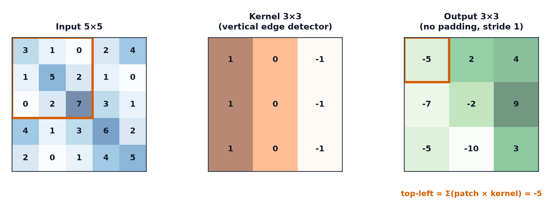
The convolution operation, step by step

Slide a small filter (e.g. $3\times3$) across the image; at each position, compute the elementwise product between the filter and the underlying image patch, then sum — that sum becomes one output pixel. Repeat across every valid position to produce the full output feature map.

Kernels as learnable feature detectors

The filter (kernel) values are learned parameters, exactly like a fully-connected layer's weights — but a single kernel is reused at every spatial position, rather than each position getting its own independent set of weights.

Classic hand-designed kernels, as intuition

The operation is fixed; only the nine numbers change. Classical vision hand-designed these kernels — a CNN learns them from data instead, which is the whole shift the architecture represents.

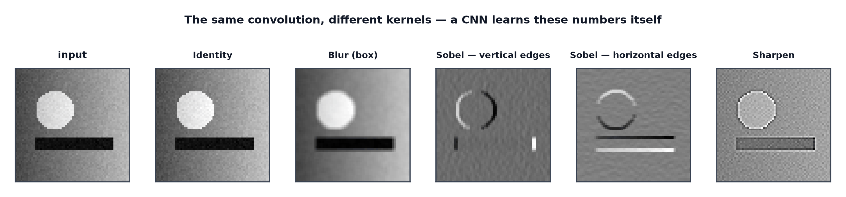
Before learned kernels, image processing used hand-designed ones: an edge-detection kernel (a small matrix approximating a spatial derivative) highlights sharp intensity changes; a blur kernel (a small uniform-averaging matrix) smooths the image; a sharpen kernel amplifies local contrast. Learned kernels in a trained CNN often converge to something visually resembling these classic edge/blob detectors in the earliest layers — a useful sanity check that the network has learned something sensible.

Stride, padding, and the output-size formula

$$n_{\text{out}} = \left\lfloor \frac{n_{\text{in}} + 2p - k}{s} \right\rfloor + 1$$

Stride $s$: how many pixels the filter moves between applications (stride 2 skips every other position, halving the output resolution). Padding $p$: pixels of border added around the input (typically zeros) before convolving, controlling whether output size shrinks (no padding) or matches input size ("same" padding).

Symbol	Meaning
$n_{\text{in}}, n_{\text{out}}$	input and output spatial size (per dimension)
$k$	kernel size
$s$	stride
$p$	padding

Multiple input and output channels

A real convolutional layer has $C_{\text{in}}$ input channels and produces $C_{\text{out}}$ output channels — each output channel is produced by its own set of $C_{\text{in}}$ kernels (one per input channel, summed together), so the total parameter count is $k \times k \times C_{\text{in}} \times C_{\text{out}}$ — this is where the overwhelming majority of a CNN's parameters actually live.

Receptive field

Each 3×3 convolution widens the receptive field by 2. Stacking three of them sees the same 7×7 region as one 7×7 kernel, using fewer parameters and inserting two extra non-linearities along the way.

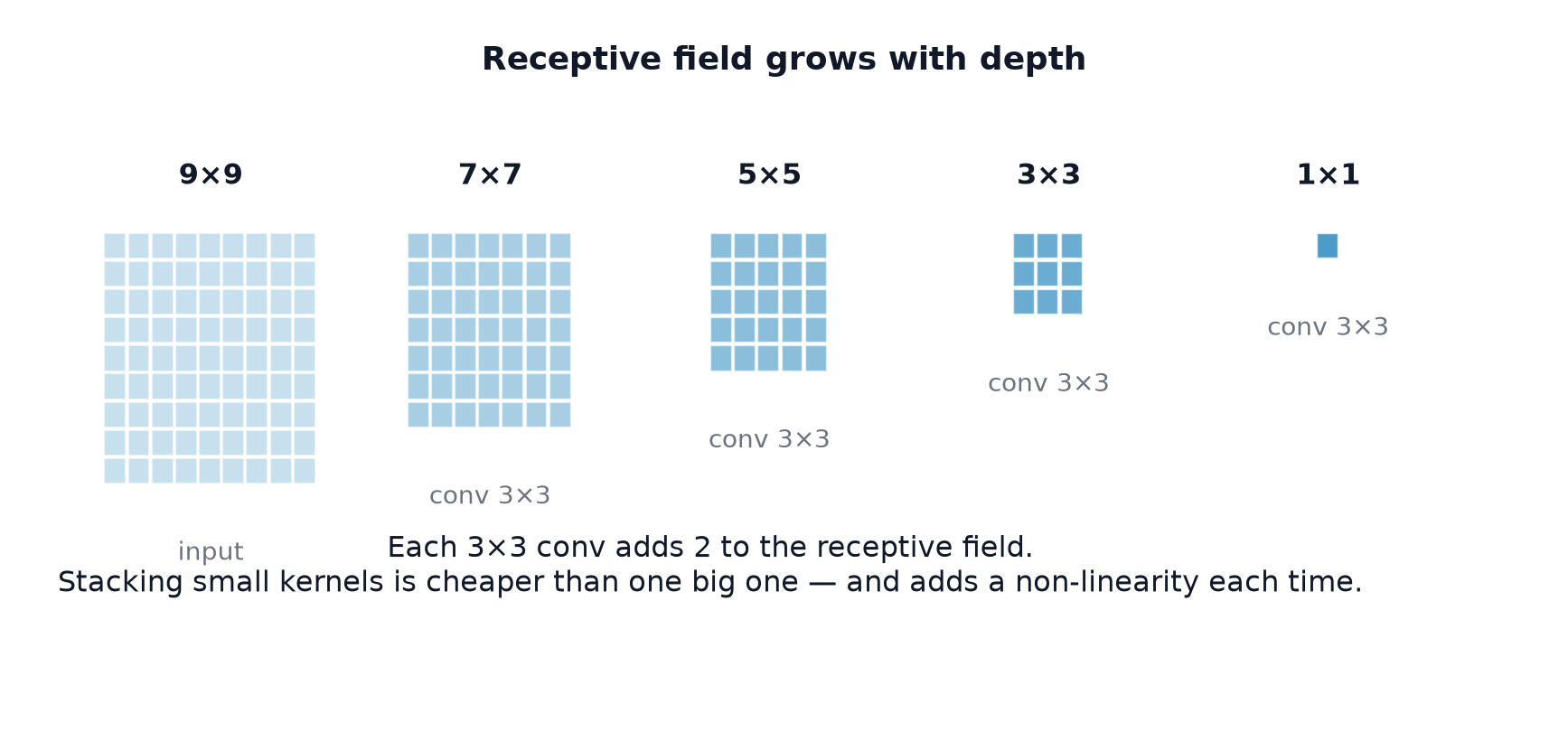
The region of the original input that a given output unit's value depends on. A single layer's receptive field equals its kernel size, but receptive field grows with depth — stacking layers lets deep units respond to increasingly large regions of the input, even though each individual layer only looks at a small local neighbourhood.

Translation equivariance vs. invariance

Equivariance: shifting the input shifts the feature map output by the same amount — a direct, provable consequence of using the identical kernel at every position. Invariance: the final prediction doesn't change when the input shifts — a stronger property that convolution alone doesn't provide, but that pooling (see Pooling and Shape Arithmetic) and global aggregation later in the network help approximate.

1×1 convolutions as channel mixing

A $1\times1$ kernel has no spatial extent at all — it operates purely across channels at each spatial position independently, mixing (and optionally reducing or expanding) the channel dimension without touching spatial structure. Used extensively to control parameter count and computation in deeper architectures.

Dilated convolutions

Insert gaps between kernel elements (a "dilation rate" $>1$), expanding the receptive field without increasing the kernel's parameter count or adding extra layers — a way to see more context cheaply, at the cost of skipping some intermediate positions entirely.

Depthwise separable convolutions

Factor a standard convolution into two cheaper steps: a depthwise convolution (one filter per input channel, no channel mixing) followed by a pointwise ($1\times1$) convolution (channel mixing, no spatial extent) — approximates a standard convolution's function at a fraction of the parameters and compute, the key trick behind mobile-oriented architectures like MobileNet (CNN Architectures).

Transposed convolution for upsampling

Sometimes called "deconvolution" (a somewhat misleading name — it is not the mathematical inverse of convolution), this operation increases spatial resolution rather than decreasing it, used throughout Semantic and Instance Segmentation's decoder path to recover full-resolution output from a compressed representation.

Code: 2-D convolution from scratch, hand-written kernels, output-size verification

convolution_demo.py

import numpy as np
import matplotlib.pyplot as plt
from PIL import Image
import torch.nn as nn
import torch

def conv2d(image, kernel):
    kh, kw = kernel.shape
    h, w = image.shape
    out_h, out_w = h - kh + 1, w - kw + 1
    output = np.zeros((out_h, out_w))
    for i in range(out_h):
        for j in range(out_w):
            output[i, j] = np.sum(image[i:i+kh, j:j+kw] * kernel)
    return output

# --- A synthetic image with a clear edge, standing in for the section's running image ---
image = np.zeros((50, 50))
image[:, 25:] = 1.0  # a vertical edge down the middle

edge_kernel = np.array([[-1, 0, 1], [-1, 0, 1], [-1, 0, 1]])  # vertical edge detector
blur_kernel = np.ones((3, 3)) / 9

edges = conv2d(image, edge_kernel)
blurred = conv2d(image, blur_kernel)

fig, axes = plt.subplots(1, 3, figsize=(12, 4))
axes[0].imshow(image, cmap="gray"); axes[0].set_title("original")
axes[1].imshow(edges, cmap="gray"); axes[1].set_title("edge kernel")
axes[2].imshow(blurred, cmap="gray"); axes[2].set_title("blur kernel")
plt.savefig("convolution_kernels.png")

# --- Output-size formula verified against torch.nn.Conv2d ---
print("n_in | kernel | stride | padding | formula | actual")
for n_in, k, s, p in [(32, 3, 1, 0), (32, 3, 1, 1), (32, 3, 2, 1), (32, 5, 2, 2)]:
    formula = (n_in + 2*p - k) // s + 1
    conv = nn.Conv2d(1, 1, kernel_size=k, stride=s, padding=p)
    actual = conv(torch.randn(1, 1, n_in, n_in)).shape[-1]
    print(f"{n_in:4d} | {k:6d} | {s:6d} | {p:7d} | {formula:7d} | {actual:6d}")

See also

• Images as Tensors — the tensor format this operation is applied to.
• Pooling and Shape Arithmetic — the companion operation for downsampling spatial resolution.