Object Detection
Classification answers "what is in this image?" Detection answers a harder question: what is in this image, where exactly is it, and how many are there? That extra "where" and "how many" is precisely what a plain classifier cannot provide, and the entire design space of detection architectures is really about different ways to propose candidate locations.
Detection reframes classification as "classify plus regress a box", and the whole design space is about how you propose the boxes.
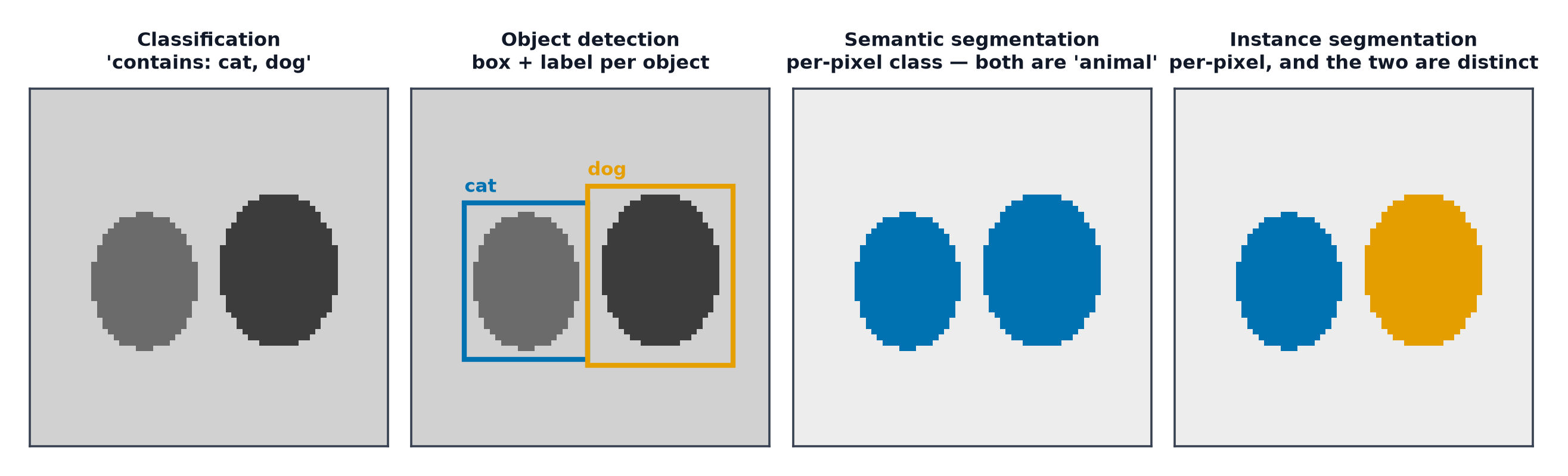
The task, and why a classifier alone cannot do it
A classifier outputs one label for the whole image, with no notion of location or count — it cannot say "there are three dogs, here, here, and here." Detection needs, per object, both a class label and a bounding box, and needs to handle a variable, unknown number of objects per image.
Bounding-box formats, and the conversion bugs
xyxy: (x_min, y_min, x_max, y_max) — the top-left and bottom-right corners. xywh: (x_center, y_center, width, height) — centre point plus size. Normalised: coordinates as fractions of image dimensions (0 to 1) rather than raw pixels, making the format independent of image resolution. Converting between these incorrectly — swapping width/height, mixing normalised and pixel coordinates — is a routine, easy-to-miss source of silently wrong training data.
Intersection over Union (IoU)
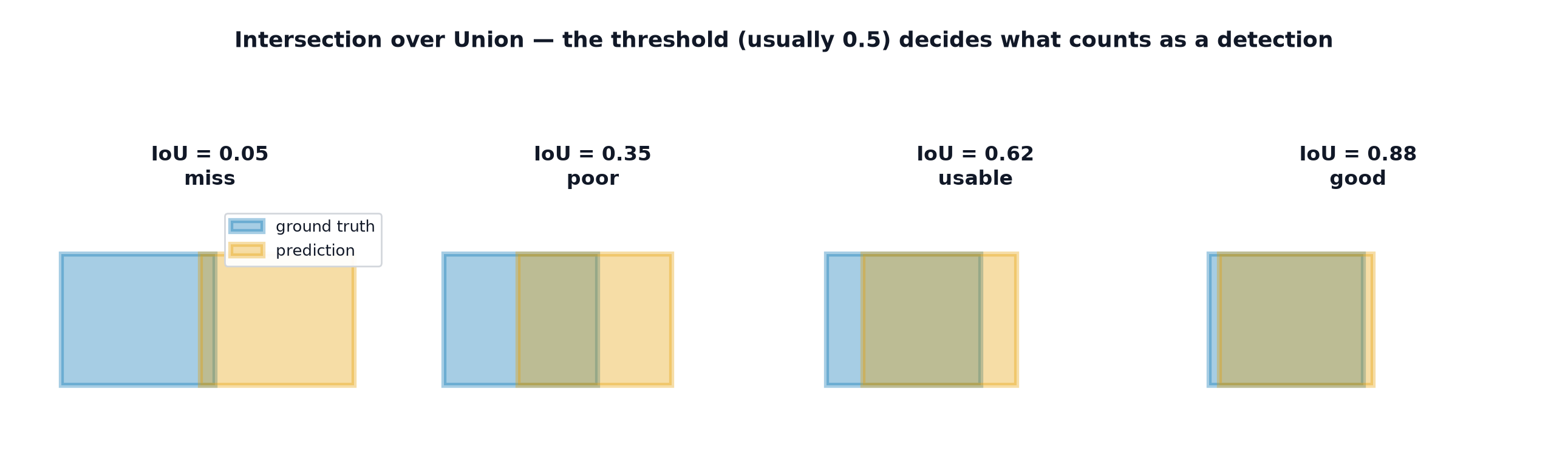
The standard measure of how well a predicted box matches a ground-truth box — 0 for no overlap, 1 for a perfect match. Used both as a training-time matching criterion (which predicted box corresponds to which ground-truth box) and as an evaluation threshold (a prediction only counts as correct if its IoU with the matching ground truth exceeds some threshold, typically 0.5).
Sliding windows, and their cost
The most naive approach: run a classifier at every position and scale within the image — correct in principle, but computationally prohibitive at the resolution and scale range real detection tasks need.
Two-stage detectors: R-CNN family
R-CNN: generate candidate regions via a separate, non-learned proposal algorithm, then run a full CNN classifier on each cropped region independently — correct but extremely slow, since the CNN reruns from scratch on every single proposal. Fast R-CNN: run the CNN backbone once over the whole image, then extract per-region features from the resulting shared feature map — far faster, since the expensive convolutional computation is no longer repeated per proposal. Faster R-CNN: replace the separate, non-learned proposal algorithm with a learned Region Proposal Network integrated directly into the model — the whole pipeline becomes trainable end to end.
One-stage detectors: YOLO and SSD
Rather than a separate proposal stage, predict boxes and classes directly, in a single forward pass, from a dense grid over the image — substantially faster than two-stage detectors, historically at some accuracy cost, though that gap has narrowed considerably in more recent one-stage designs.
Anchor boxes
Pre-defined reference boxes of various sizes and aspect ratios, tiled across the image at every grid position — rather than predicting a box's absolute coordinates from scratch, the model predicts offsets relative to the nearest matching anchor, which is generally an easier learning target than raw coordinate regression.
Anchor-free detectors
Predict object centres (and their extent) directly, without any predefined anchor boxes — removes the anchor-design hyperparameters (how many, what sizes, what aspect ratios) that anchor-based methods need carefully tuned, at the cost of a different set of design choices for defining what counts as an object "centre."
DETR and set prediction with transformers
Reframes detection as a direct set prediction problem: a transformer (see Transformer Architecture) attends over the image and outputs a fixed-size set of predictions directly, matched to ground-truth objects via an optimal bipartite matching during training — eliminates both anchor boxes and the separate non-maximum-suppression post-processing step below, at the cost of typically slower convergence during training.
Non-maximum suppression (NMS)
A detector typically produces many overlapping candidate boxes for the same object. NMS removes near-duplicates: sort by confidence, keep the highest-confidence box, discard any remaining box whose IoU with a kept box exceeds a threshold, repeat — reduces the raw prediction set down to (ideally) one box per actual object.
The detection loss
A combination of a classification loss (cross-entropy, as in Loss Functions) for the predicted class, and a localisation/regression loss (e.g. smooth L1) for the predicted box coordinates, weighted together.
| Symbol | Meaning |
|---|---|
| IoU | Intersection over Union between two boxes |
| weight balancing classification against localisation loss |
mAP explained properly
Average Precision (AP) for one class: the area under that class's precision-recall curve (from Evaluation Metrics for Classification), computed at a specific IoU threshold defining what counts as a correct detection. mAP: the mean of AP across all classes. mAP@[.5:.95]: AP averaged not just across classes but across a range of IoU thresholds (0.5 to 0.95, in steps), rewarding models whose boxes are precisely, not just roughly, correct.
Speed/accuracy comparison table
| Two-stage (Faster R-CNN) | One-stage (YOLO/SSD) | DETR | |
|---|---|---|---|
| Speed | slower | faster | moderate |
| Accuracy | historically higher | competitive in recent versions | competitive, especially on large objects |
| Post-processing | NMS required | NMS required | none (set prediction) |
| Training convergence | moderate | fast | slow |
Code: IoU and NMS from scratch, a pretrained detector on the running image
import numpy as np
import torch
from torchvision.models.detection import fasterrcnn_resnet50_fpn, FasterRCNN_ResNet50_FPN_Weights
from PIL import Image
import matplotlib.pyplot as plt
import matplotlib.patches as patches

def iou(box1, box2):
    x1, y1 = max(box1[0], box2[0]), max(box1[1], box2[1])
    x2, y2 = min(box1[2], box2[2]), min(box1[3], box2[3])
    intersection = max(0, x2 - x1) * max(0, y2 - y1)
    area1 = (box1[2]-box1[0]) * (box1[3]-box1[1])
    area2 = (box2[2]-box2[0]) * (box2[3]-box2[1])
    return intersection / (area1 + area2 - intersection + 1e-8)

def nms(boxes, scores, iou_threshold=0.5):
    order = np.argsort(scores)[::-1]
    keep = []
    while len(order) > 0:
        i = order[0]
        keep.append(i)
        order = order[1:]
        order = [j for j in order if iou(boxes[i], boxes[j]) < iou_threshold]
    return keep

boxes = np.array([[10, 10, 50, 50], [12, 12, 52, 52], [100, 100, 150, 150]])
scores = np.array([0.9, 0.85, 0.95])
kept = nms(boxes, scores)
print("boxes before NMS:", len(boxes), " boxes after NMS:", len(kept), " kept indices:", kept)

# --- Pretrained Faster R-CNN on the running image ---
rng = np.random.default_rng(0)
img_array = rng.integers(0, 256, size=(224, 224, 3), dtype=np.uint8)
img_tensor = torch.tensor(img_array).permute(2, 0, 1).float() / 255.0

model = fasterrcnn_resnet50_fpn(weights=FasterRCNN_ResNet50_FPN_Weights.DEFAULT)
model.eval()
with torch.no_grad():
    predictions = model([img_tensor])[0]

fig, ax = plt.subplots()
ax.imshow(img_array)
for box, score in zip(predictions["boxes"][:5], predictions["scores"][:5]):
    x1, y1, x2, y2 = box.tolist()
    rect = patches.Rectangle((x1, y1), x2-x1, y2-y1, fill=False, edgecolor="red")
    ax.add_patch(rect)
    ax.text(x1, y1, f"{score:.2f}", color="red")
plt.savefig("detection_boxes.png")
See also
- Semantic and Instance Segmentation — the pixel-level generalisation of the box-level task this page covers.
- Evaluation Metrics for Classification — the precision/recall machinery mAP is built on.