Pooling and Shape Arithmetic
A CNN's spatial resolution has to shrink somewhere between a 224×224 input and a single classification decision — pooling is the classic way to do that shrinking, trading spatial precision for a degree of invariance and reduced compute. Getting the resulting shapes right, at every layer, is the single most useful bookkeeping habit for building a CNN that actually runs.
Pooling trades spatial precision for invariance and compute, and modern architectures increasingly do it with strided convolutions instead.
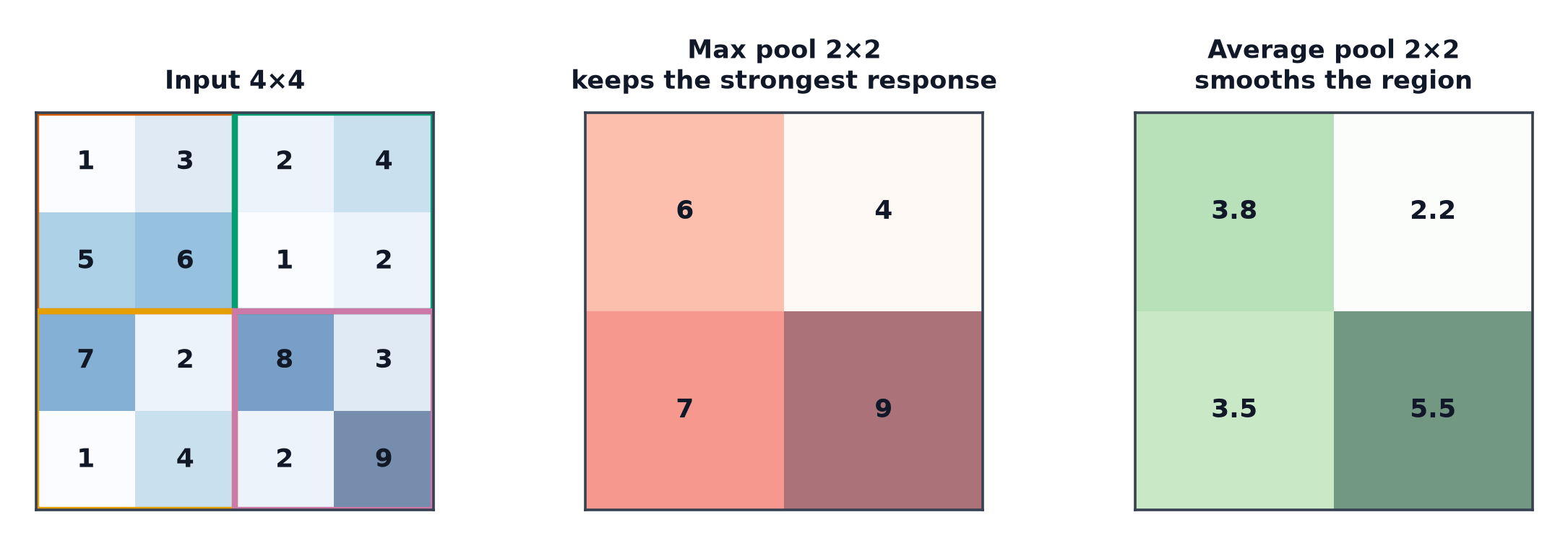
Max pooling
Slide a window (e.g. ) across the feature map, keeping only the maximum value in each window — reduces spatial resolution while preserving the strongest activation in each local region, the assumption being that the strongest response is the most informative one.
Average pooling
The same sliding-window idea, but averaging instead of taking the max — smoother, less prone to being dominated by a single outlier activation, but also less selective about which features survive.
The invariance argument, and its limits
If a feature shifts by a small amount within a pooling window, max pooling's output is unchanged (the same maximum value survives regardless of exactly where within the window it occurred) — a modest degree of local translation invariance. The limit: this invariance only holds within one pooling window's extent; a shift larger than the window still changes the output.
Pooling vs. strided convolution
A convolution with stride (from The Convolution Operation) also downsamples spatial resolution, but does so via a learned operation rather than a fixed max/average rule — many modern architectures have replaced explicit pooling layers with strided convolutions throughout, on the reasoning that a learned downsampling operation can adapt to the task rather than applying the same fixed rule everywhere.
Global average pooling
Average an entire feature map (across all spatial positions) down to a single value per channel — replacing the large fully-connected classification head that early CNNs used (which held a disproportionate share of total parameters) with a much smaller, nearly parameter-free operation, directly connecting the final convolutional feature maps to the class predictions.
Adaptive pooling for variable input sizes
Rather than a fixed window size, adaptive pooling specifies the desired output size directly, and the layer automatically computes whatever window/stride achieves it — lets the same architecture accept input images of varying sizes and still produce a fixed-size feature map for the classification head, without manually recomputing pooling parameters per input size.
A complete shape-arithmetic walkthrough
| Layer | Operation | Output shape |
|---|---|---|
| Input | — | |
| Conv, | ||
| MaxPool, | ||
| Conv, | same-padding, unchanged | |
| MaxPool, | ||
| GlobalAvgPool | average over | |
| Linear | project to classes |
| Symbol | Meaning |
|---|---|
| kernel size, stride, padding — same conventions as The Convolution Operation |
Computing the flatten dimension without guessing
Before global average pooling became standard, connecting a convolutional feature map to a fully-connected layer required manually flattening it — and computing that flattened size by hand (multiplying channels × height × width after every prior layer's shape change) is error-prone. The reliable approach: pass a dummy input tensor through the convolutional layers programmatically and read .shape directly, rather than computing it by hand.
Receptive field of the whole network
Summing the effective receptive field contributed by every convolution and pooling layer in sequence gives the final receptive field — the region of the original input image that the network's very last feature map position depends on; a network whose final receptive field doesn't cover the whole input image cannot use global context in its last layer.
The classic shape-mismatch errors, and how to read them
RuntimeError: mat1 and mat2 shapes cannot be multiplied (a fully-connected layer's expected input size doesn't match the actual flattened feature map size — almost always because a prior conv/pool layer's output shape wasn't recomputed after a change) and RuntimeError: Given input size ... calculated output size is too small (a pooling window larger than the remaining spatial dimensions at that point in a deep network) are the two most common shape errors in a CNN, and both are located immediately by printing shapes layer by layer.
Code: shape hook, flatten dimension computed programmatically, a mismatch caught
import torch
import torch.nn as nn

class SimpleCNN(nn.Module):
    def __init__(self, num_classes=10):
        super().__init__()
        self.features = nn.Sequential(
            nn.Conv2d(3, 32, kernel_size=3, padding=1), nn.ReLU(), nn.MaxPool2d(2),
            nn.Conv2d(32, 64, kernel_size=3, padding=1), nn.ReLU(), nn.MaxPool2d(2),
            nn.Conv2d(64, 128, kernel_size=3, padding=1), nn.ReLU(), nn.AdaptiveAvgPool2d(1),
        )
        # compute the flatten dimension programmatically, never by hand
        with torch.no_grad():
            dummy = torch.zeros(1, 3, 64, 64)
            flat_dim = self.features(dummy).flatten(1).shape[1]
        self.classifier = nn.Linear(flat_dim, num_classes)

    def forward(self, x):
        x = self.features(x)
        x = x.flatten(1)
        return self.classifier(x)

model = SimpleCNN()

# --- Forward hook printing the shape after every layer ---
def make_hook(name):
    def hook(module, input, output):
        print(f"{name:20s}: {tuple(output.shape)}")
    return hook

for name, layer in model.features.named_children():
    layer.register_forward_hook(make_hook(f"features.{name}"))

output = model(torch.randn(2, 3, 64, 64))
print("final output shape:", output.shape)

# --- A deliberate mismatch: a pooling window too large for the remaining spatial size ---
try:
    broken = nn.Sequential(
        nn.Conv2d(3, 16, kernel_size=3), nn.MaxPool2d(20),  # window far larger than what remains
    )
    broken(torch.randn(1, 3, 16, 16))
except RuntimeError as e:
    print(f"\ncaught the expected shape error: {e}")
See also
- The Convolution Operation — the operation this page's downsampling complements.
- CNN Architectures — the full architectures assembled from these two building blocks.