Semantic and Instance Segmentation

Object Detection draws a rectangle around an object. Segmentation is more demanding still: classify every single pixel. The architecture this demands has a distinctive shape — downsample to understand what's in the image, then upsample back to full resolution to say exactly where — and the skip connections carrying detail across that shape are the entire design.

Key idea

Segmentation networks are encoder-decoders - downsample to understand, upsample to localise, and skip connections carry back the spatial detail lost on the way down.

Semantic segmentation assigns a class to every pixel; instance segmentation additionally separates individual objects of that class. The distinction only matters when objects of the same class touch — which in practice is most of the time.

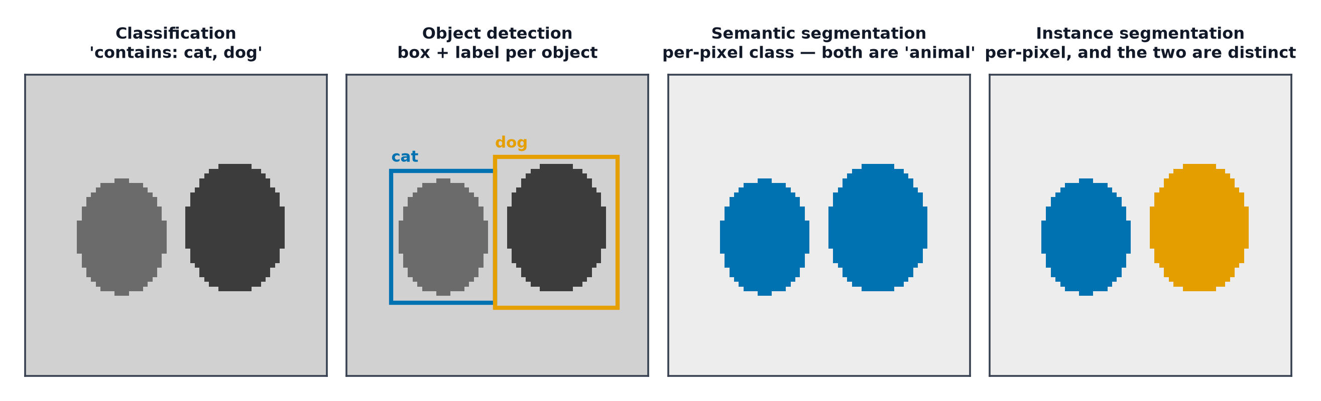
Semantic vs. instance vs. panoptic segmentation

Semantic segmentation: every pixel gets a class label, but distinct objects of the same class aren't distinguished (all "car" pixels are just "car," whether from one car or five). Instance segmentation: distinguishes individual object instances — each car gets its own separate mask, extending Object Detection's per-object framing down to pixel precision. Panoptic segmentation: combines both — every pixel gets a class label, and object-class pixels are additionally split into distinct instances.

The output shape

Where a classifier outputs one label for the whole image, a semantic segmentation model outputs a full class map matching the input's spatial resolution — one class label per pixel, not one label per image.

Fully convolutional networks

Replacing a classification network's final fully-connected layers with more convolutional layers keeps the output spatially structured (a 2-D map) rather than collapsing to a single flat vector — the foundational insight that made dense, per-pixel prediction from a CNN practical at all.

The upsampling problem

A standard CNN backbone progressively downsamples spatial resolution (Pooling and Shape Arithmetic) to build abstract, low-resolution features — but segmentation needs full-resolution output. Three ways to upsample back: transposed convolution (a learned upsampling operation, from The Convolution Operation), bilinear upsampling (a fixed, non-learned interpolation), and pixel shuffle (rearranging channel-dimension values into spatial resolution, avoiding some of transposed convolution's characteristic checkerboard artefacts).

U-Net, and why the skip connections are the whole architecture

U-Net's encoder progressively downsamples (building abstract understanding), and its decoder progressively upsamples back to full resolution — but the critical piece is the skip connections directly linking each encoder resolution level to its matching decoder resolution level. Without them, fine spatial detail lost during downsampling (exact edges, precise boundaries) simply cannot be recovered by the decoder alone, no matter how it upsamples — the skip connections are what let the output have both the encoder's semantic understanding and the input's precise spatial detail.

Encoder-decoder with a pretrained backbone

Rather than training the encoder half from scratch, a pretrained classification backbone (Transfer Learning for Vision) can serve as the encoder directly — the decoder (with its skip connections) is added on top and trained (or fine-tuned) for the segmentation task, combining transfer learning's benefits with U-Net's architecture.

Mask R-CNN for instance masks

Extends Object Detection's Faster R-CNN with an additional branch predicting a pixel mask within each detected bounding box — detection and instance segmentation share the same underlying region-proposal machinery, with the mask branch adding pixel-level precision on top of the box-level detection.

Segmentation losses

Pixel cross-entropy: standard classification loss (Loss Functions), applied independently at every pixel. Dice loss: directly optimises the Dice coefficient (below), often more robust than pixel cross-entropy when the target class occupies a small fraction of the image. Focal loss: from Loss Functions, down-weights easy (already well-classified) pixels — combinations of these losses (e.g. Dice + cross-entropy) are common in practice.

Class imbalance in dense prediction

In most real segmentation tasks, background pixels vastly outnumber the pixels of any specific object class — plain pixel cross-entropy, optimised naively, can be dominated by trivially getting the background right while barely learning the rare, small foreground class, exactly the Imbalanced Data problem, applied per-pixel rather than per-example.

Metrics: pixel accuracy, IoU/Jaccard, Dice, mIoU

$$\text{Dice} = \frac{2|A \cap B|}{|A| + |B|}, \qquad \text{IoU} = \frac{|A \cap B|}{|A \cup B|}$$

Pixel accuracy: fraction of correctly-classified pixels — suffers the same imbalance-driven misleading-ness as Evaluation Metrics for Classification's accuracy trap. IoU/Jaccard: Object Detection's box-overlap measure, applied to pixel masks instead of boxes. Dice: closely related to IoU, weighting overlap slightly differently, common in medical segmentation specifically. mIoU: mean IoU across all classes, the standard summary metric for semantic segmentation.

Symbol	Meaning
$A, B$	the predicted and ground-truth pixel sets for a given class

Annotation cost as the real constraint

Pixel-precise mask annotation is dramatically more expensive and time-consuming to produce than image-level labels or even bounding boxes — annotation cost, not model capability, is frequently the actual bottleneck limiting segmentation dataset size in practice, more so than for classification or detection tasks.

Code: a U-Net from scratch, Dice/IoU verified

segmentation_demo.py

import torch
import torch.nn as nn

class UNetBlock(nn.Module):
    def __init__(self, in_c, out_c):
        super().__init__()
        self.conv = nn.Sequential(
            nn.Conv2d(in_c, out_c, 3, padding=1), nn.ReLU(),
            nn.Conv2d(out_c, out_c, 3, padding=1), nn.ReLU(),
        )
    def forward(self, x): return self.conv(x)

class SmallUNet(nn.Module):
    def __init__(self, num_classes=2):
        super().__init__()
        self.enc1 = UNetBlock(3, 16); self.pool1 = nn.MaxPool2d(2)
        self.enc2 = UNetBlock(16, 32); self.pool2 = nn.MaxPool2d(2)
        self.bottleneck = UNetBlock(32, 64)
        self.up2 = nn.ConvTranspose2d(64, 32, 2, stride=2)
        self.dec2 = UNetBlock(64, 32)  # 64 = 32 (upsampled) + 32 (skip)
        self.up1 = nn.ConvTranspose2d(32, 16, 2, stride=2)
        self.dec1 = UNetBlock(32, 16)  # 32 = 16 (upsampled) + 16 (skip)
        self.out = nn.Conv2d(16, num_classes, 1)

    def forward(self, x):
        e1 = self.enc1(x); p1 = self.pool1(e1)
        e2 = self.enc2(p1); p2 = self.pool2(e2)
        b = self.bottleneck(p2)
        d2 = self.up2(b)
        d2 = self.dec2(torch.cat([d2, e2], dim=1))  # skip connection
        d1 = self.up1(d2)
        d1 = self.dec1(torch.cat([d1, e1], dim=1))  # skip connection
        return self.out(d1)

torch.manual_seed(0)
model = SmallUNet(num_classes=2)
x = torch.randn(4, 3, 64, 64)
output = model(x)
print("input shape:", x.shape, " output shape (per-pixel class logits):", output.shape)

def dice_coefficient(pred_mask, true_mask, eps=1e-8):
    intersection = (pred_mask * true_mask).sum()
    return (2 * intersection + eps) / (pred_mask.sum() + true_mask.sum() + eps)

def iou_score(pred_mask, true_mask, eps=1e-8):
    intersection = (pred_mask * true_mask).sum()
    union = pred_mask.sum() + true_mask.sum() - intersection
    return (intersection + eps) / (union + eps)

pred = (torch.rand(64, 64) > 0.5).float()
true = (torch.rand(64, 64) > 0.5).float()
print(f"Dice: {dice_coefficient(pred, true):.4f}, IoU: {iou_score(pred, true):.4f}")
print(f"Dice on identical masks (should be 1.0): {dice_coefficient(pred, pred):.4f}")

See also

• Object Detection — the box-level task this page extends to pixel precision.
• Deploying Vision Models — serving a segmentation model in production.