Vision Transformers

The architecture that took over NLP turns out to work for images too, once you accept one reframing: an image is a sequence of patches. Once that step is taken, the entire transformer stack from Transformer Architecture transfers to vision essentially unchanged — the same attention, the same feed-forward blocks, the same residual and normalisation pattern.

Key idea

An image is a sequence of patches - once you accept that, the entire transformer stack transfers unchanged.

A ViT cuts the image into fixed patches, flattens each into a vector, and feeds the result to a standard transformer. There is no convolution anywhere — the locality a CNN has built in must instead be learned from data, which is why ViTs need far more of it.

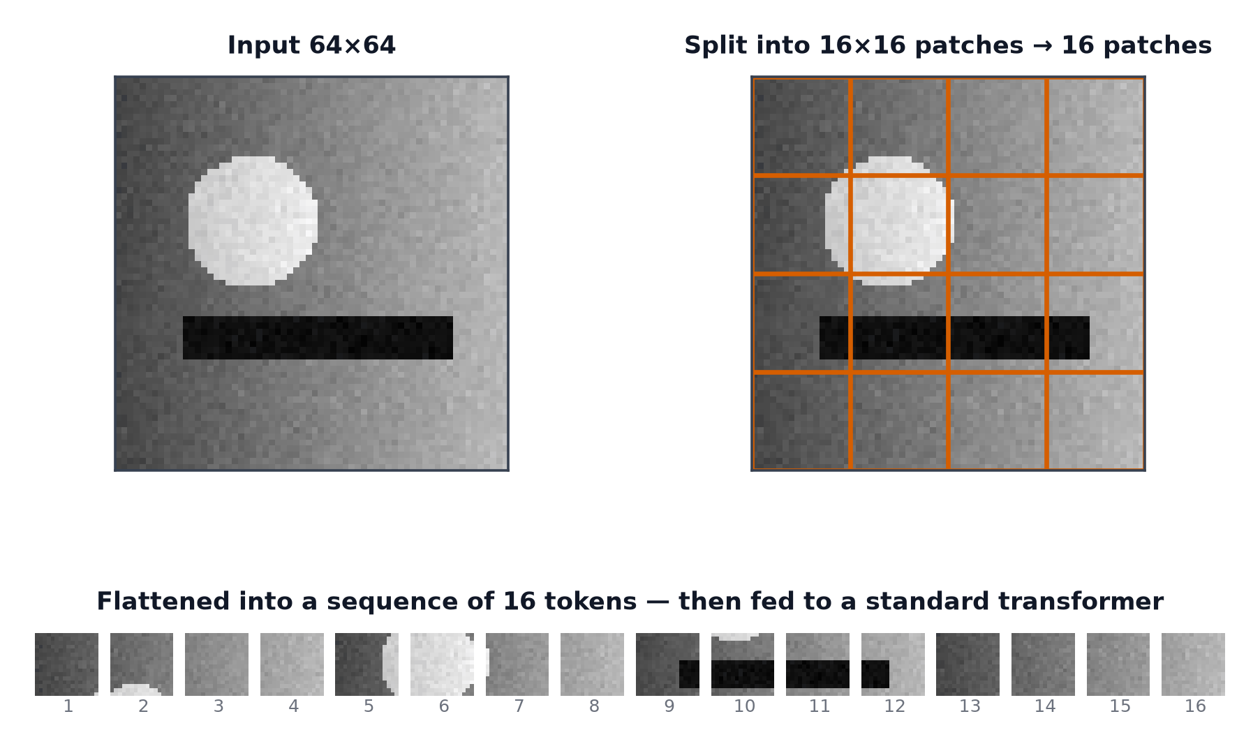
Patch embedding: split, flatten, project

Divide the image into fixed-size non-overlapping patches (e.g. $16\times16$ pixels); flatten each patch into a single vector; linearly project each flattened patch into the model's embedding dimension — the resulting sequence of patch embeddings is exactly analogous to a sequence of token embeddings in Word Embeddings.

The [CLS] token

A learnable embedding prepended to the patch sequence (borrowed directly from Pretraining Objectives's BERT convention) — after passing through the transformer, this token's final representation is used as a summary of the whole image for classification, having attended to every patch along the way.

Positional embeddings for 2-D layout

Patches, like tokens, carry no inherent order to a transformer — a learned (or occasionally fixed) positional embedding is added to each patch embedding, encoding its row/column position in the original image grid, directly analogous to Positional Encodings's treatment of sequence position.

The encoder stack, unchanged from the NLP section

Once the input is a sequence of embedded patches plus positional information, the rest is exactly Transformer Architecture's encoder: multi-head self-attention, residual connections, layer normalisation, feed-forward blocks — no vision-specific modification required.

The classification head

A simple linear layer applied to the final [CLS] token's representation, projecting to the number of target classes — the entire vision-specific part of the architecture is just this final layer and the initial patch embedding; everything in between is generic transformer machinery.

The inductive-bias trade

CNNs have locality and translation equivariance built into the convolution operation (The Convolution Operation) — a strong prior that images have local structure. Vision transformers have no such built-in prior; every patch can attend to every other patch from the very first layer, with no inherent notion that nearby patches are more related than distant ones. This means ViT must learn spatial structure entirely from data — which requires either substantially more training data or stronger augmentation than a CNN needs to reach comparable performance.

$$n = \frac{H \times W}{P^2}$$

Symbol	Meaning
$H, W$	image height and width
$P$	patch size
$n$	number of patches (sequence length for the transformer)

When ViT beats CNNs, and when it does not

With enough training data (or a sufficiently strong pretraining regime), ViT tends to match or exceed CNN performance, and scales well to very large model and data sizes. With limited data and no strong pretraining, CNNs' built-in locality bias tends to win — ViT's flexibility is an advantage only once enough data is available to actually learn what the bias would otherwise have provided for free.

Hybrid designs

Some architectures use a CNN for early, local feature extraction, then feed the resulting feature map (rather than raw pixel patches) into a transformer for later, global reasoning — combining CNN's local inductive bias with transformer's long-range attention.

Swin transformers and hierarchical windows

Rather than full attention across all patches (with $O(n^2)$ cost in patch count, from Self-Attention in Depth), Swin restricts attention to local windows most of the time, shifting the window boundaries between layers so information still eventually propagates across the whole image — produces a hierarchical, multi-resolution feature structure closer to a CNN's, at reduced computational cost relative to full ViT attention.

DeiT and distillation-based data efficiency

Addresses ViT's large-data requirement directly: train a smaller ViT using knowledge distillation from a strong CNN teacher — the CNN's built-in inductive bias is transferred indirectly through the distillation signal, letting the ViT student reach strong performance with substantially less training data than training a ViT from scratch would need.

Attention maps as a partial interpretability tool

Visualising which patches the [CLS] token (or other patches) attend to most strongly can highlight image regions the model found relevant — a genuinely useful diagnostic, subject to the same caveat as Self-Attention in Depth's discussion: attention weights are suggestive evidence, not a complete or fully reliable explanation of the model's decision.

Comparison against CNNs

	CNN	ViT
Inductive bias	strong (locality, equivariance)	weak/none, learned from data
Data efficiency	good with limited data	needs more data or strong pretraining
Compute scaling	well-understood, efficient	scales well with data+compute at large scale
Long-range dependencies	limited (bounded by receptive field)	native, from the first layer

Code: patch embedding from scratch, a small ViT block, attention map

vision_transformers_demo.py

import torch
import torch.nn as nn
import numpy as np
import matplotlib.pyplot as plt

def patchify(image, patch_size):
    C, H, W = image.shape
    patches = image.unfold(1, patch_size, patch_size).unfold(2, patch_size, patch_size)
    patches = patches.contiguous().view(C, -1, patch_size, patch_size)
    return patches.permute(1, 0, 2, 3).flatten(1)  # (n_patches, C*P*P)

rng = np.random.default_rng(0)
image = torch.tensor(rng.integers(0, 256, size=(3, 64, 64)), dtype=torch.float32) / 255.0
patch_size = 16
patches = patchify(image, patch_size)
print(f"image shape: {tuple(image.shape)} -> {patches.shape[0]} patches of dim {patches.shape[1]}")

fig, axes = plt.subplots(4, 4, figsize=(6, 6))
for i, ax in enumerate(axes.flat):
    patch_img = patches[i].view(3, patch_size, patch_size).permute(1, 2, 0)
    ax.imshow(patch_img); ax.axis("off")
plt.savefig("patch_grid.png")

# --- A minimal ViT block, reusing the transformer encoder block ---
class MinimalViT(nn.Module):
    def __init__(self, patch_dim, d_model, n_heads, n_patches, num_classes):
        super().__init__()
        self.proj = nn.Linear(patch_dim, d_model)
        self.cls_token = nn.Parameter(torch.randn(1, d_model))
        self.pos_embed = nn.Parameter(torch.randn(n_patches + 1, d_model))
        self.encoder = nn.TransformerEncoderLayer(d_model, n_heads, batch_first=True, norm_first=True)
        self.head = nn.Linear(d_model, num_classes)

    def forward(self, patch_seq):
        x = self.proj(patch_seq)
        cls = self.cls_token.expand(x.shape[0], 1, -1)
        x = torch.cat([cls, x], dim=1) + self.pos_embed
        x = self.encoder(x)
        return self.head(x[:, 0])  # [CLS] token's final representation

vit = MinimalViT(patch_dim=patches.shape[1], d_model=32, n_heads=4, n_patches=patches.shape[0], num_classes=10)
logits = vit(patches.unsqueeze(0))
print("ViT output shape (class logits):", logits.shape)

See also

• Transformer Architecture — the unmodified architecture this page applies to images.
• CNN Architectures — the built-in-inductive-bias alternative ViT trades away.