Activation Functions

The non-linearity between layers is what makes depth meaningful at all — From Perceptron to MLP proved that a stack of purely linear layers collapses into a single linear layer. But not all non-linearities are equal: the shape of an activation's derivative determines whether gradients survive a deep network or vanish before reaching the early layers.

Key idea

An activation is chosen for the shape of its derivative as much as for the shape of itself — saturation is what kills training.

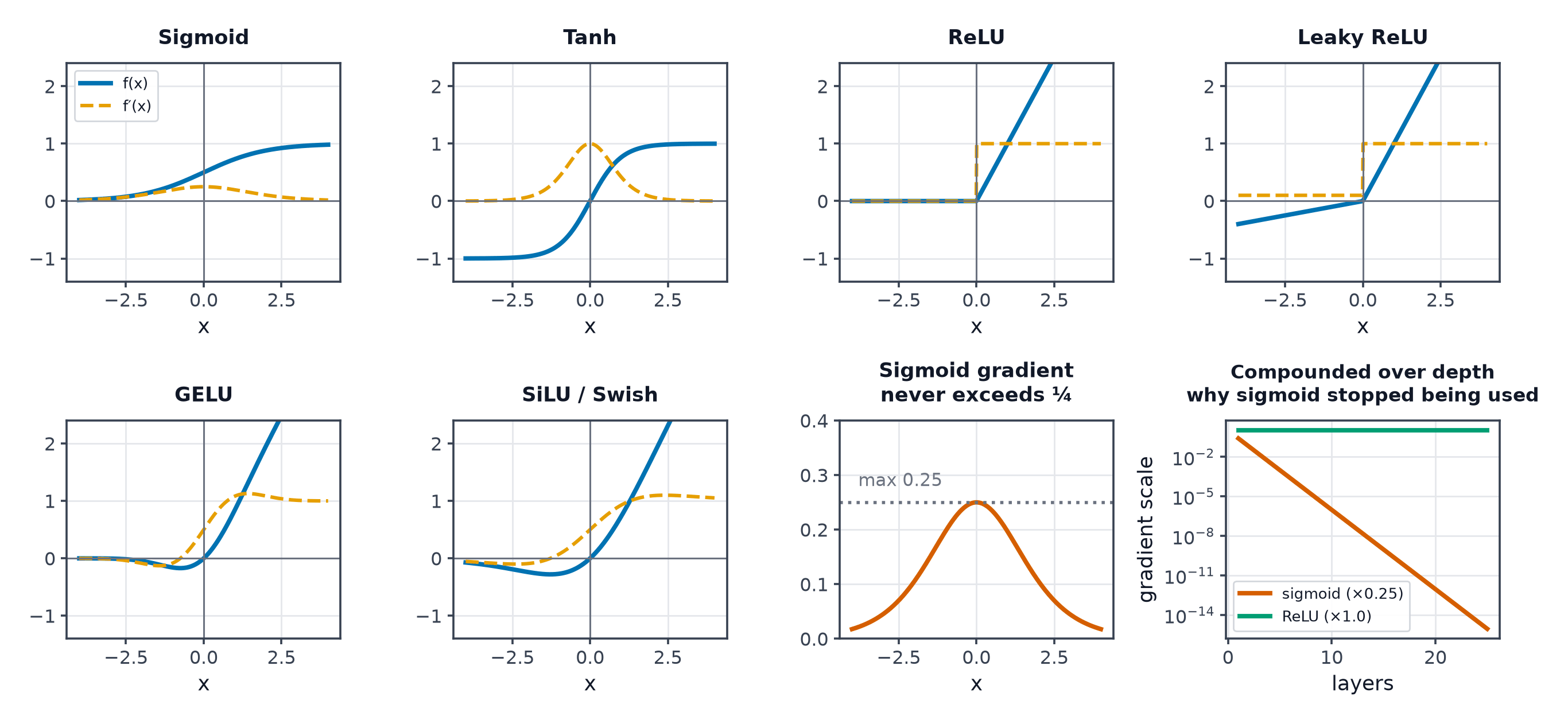
Each activation with its derivative dashed. The bottom-right panels are the reason ReLU displaced sigmoid: the sigmoid's gradient never exceeds ¼, so twenty stacked layers multiply the signal by at most 4⁻²⁰.

Sigmoid

$$\sigma(z) = \frac{1}{1+e^{-z}}, \qquad \sigma'(z) = \sigma(z)(1-\sigma(z))$$

Range $(0,1)$. Saturation: for large $|z|$, $\sigma'(z) \to 0$ — the derivative flattens to nearly zero far from the origin, which means gradients flowing through a saturated sigmoid unit are multiplied by a near-zero number, contributing to Vanishing and Exploding Gradients. Its maximum derivative value is only 0.25 (at $z=0$), meaning even a healthy sigmoid unit shrinks gradients by at least 4x on every pass through it.

Tanh

$$\tanh(z) = \frac{e^z - e^{-z}}{e^z + e^{-z}}, \qquad \tanh'(z) = 1 - \tanh^2(z)$$

Range $(-1,1)$, zero-centred (unlike sigmoid) — a genuine improvement, since zero-centred activations don't systematically bias the sign of downstream gradients. Still saturates at the extremes, with the same vanishing-gradient problem as sigmoid, just with a larger maximum derivative (1.0 at $z=0$ vs. sigmoid's 0.25).

ReLU

$$\text{ReLU}(z) = \max(0, z), \qquad \text{ReLU}'(z) = \begin{cases} 1 & z > 0 \\ 0 & z \le 0 \end{cases}$$

Cheap (no exponential), non-saturating on the positive side (derivative is exactly 1, not shrinking, for any positive input) — this is the single biggest reason ReLU displaced sigmoid/tanh as the default. Dying ReLU: a unit whose weights push it to always output a negative pre-activation gets a permanent zero gradient and stops learning entirely — once dead, a ReLU unit typically never recovers, since its gradient is zero regardless of the input.

Leaky ReLU, PReLU, ELU

• Leaky ReLU: $\max(\alpha z, z)$ with small $\alpha$ (e.g. 0.01) — allows a small gradient for negative inputs, addressing dying ReLU directly.
• PReLU: same shape, but $\alpha$ is a learned parameter rather than fixed.
• ELU: smooth for negative inputs ($\alpha(e^z - 1)$), approaching $-\alpha$ asymptotically rather than a hard linear slope — can produce negative outputs with a smoother gradient than Leaky ReLU near zero.

GELU and SiLU/Swish

$$\text{GELU}(z) = z \cdot \Phi(z), \qquad \text{SiLU}(z) = z \cdot \sigma(z)$$

where $\Phi$ is the standard Gaussian CDF. Both are smooth, non-monotonic (they dip slightly negative before rising) approximations to a "soft gate" on the input. Transformers (Transformer Architecture) predominantly use GELU (or SiLU-family variants) rather than ReLU — empirically smoother optimisation landscapes, though the precise reason remains an active research question rather than a settled theoretical result.

Softmax as an output layer, not a hidden activation

$$\text{softmax}(z)_k = \frac{e^{z_k}}{\sum_j e^{z_j}}$$

Converts a vector of scores into a probability distribution — used for multi-class output layers (Logistic Regression's multi-class generalisation) and inside Attention Mechanism, but never as a hidden-layer activation, since it couples all units together (each output depends on every input), unlike the elementwise activations above.

Activation	Derivative	Range	Saturates?
Sigmoid	$\sigma(1-\sigma)$	$(0,1)$	both sides
Tanh	$1-\tanh^2$	$(-1,1)$	both sides
ReLU	1 or 0	$[0,\infty)$	negative side only (dies)
Leaky ReLU	1 or $\alpha$	$(-\infty,\infty)$	no
GELU/SiLU	smooth, non-monotonic	$\approx(-0.2,\infty)$	no

Numerical stability of softmax

Computed naively, $e^{z_k}$ overflows for even moderately large $z_k$. The standard fix subtracts the max before exponentiating: $\text{softmax}(z)_k = \frac{e^{z_k - \max(z)}}{\sum_j e^{z_j - \max(z)}}$ — mathematically identical (the max cancels in numerator and denominator) but numerically stable.

Selection table

Architecture	Default activation
MLP / CNN hidden layers	ReLU (or a variant if dying ReLU is observed)
Transformer feed-forward blocks	GELU or SiLU
Output layer, binary classification	sigmoid
Output layer, multi-class classification	softmax
Output layer, regression	none (linear)

Code: plotting every activation and its derivative, softmax stability, dying ReLU

activation_functions_demo.py

import numpy as np
import matplotlib.pyplot as plt

z = np.linspace(-6, 6, 200)

def sigmoid(z): return 1 / (1 + np.exp(-z))
def relu(z): return np.maximum(0, z)
def gelu(z):
    from scipy.stats import norm
    return z * norm.cdf(z)

activations = {
    "sigmoid": (sigmoid(z), sigmoid(z) * (1 - sigmoid(z))),
    "tanh": (np.tanh(z), 1 - np.tanh(z) ** 2),
    "relu": (relu(z), (z > 0).astype(float)),
    "gelu": (gelu(z), np.gradient(gelu(z), z)),
}

fig, axes = plt.subplots(2, len(activations), figsize=(16, 6))
for i, (name, (act, deriv)) in enumerate(activations.items()):
    axes[0, i].plot(z, act); axes[0, i].set_title(name)
    axes[1, i].plot(z, deriv); axes[1, i].set_title(f"{name} derivative")
plt.savefig("activations_and_derivatives.png")

# --- Numerically stable vs naive softmax ---
def naive_softmax(z):
    exp = np.exp(z)
    return exp / exp.sum()

def stable_softmax(z):
    exp = np.exp(z - z.max())
    return exp / exp.sum()

big_logits = np.array([1000.0, 1001.0, 1002.0])
print("naive softmax:", naive_softmax(big_logits), "  <- nan, overflow")
print("stable softmax:", stable_softmax(big_logits), "  <- correct")

# --- Dying ReLU: count dead units after biasing weights very negative ---
rng = np.random.default_rng(0)
W = rng.normal(size=(50, 200))
X = rng.normal(size=(1000, 50))
z_bad_init = X @ (W - 5.0)  # pushed strongly negative
activations_out = relu(z_bad_init)
dead_units = np.mean(np.all(activations_out == 0, axis=0))
print(f"fraction of dead ReLU units under bad init: {dead_units:.2%}")

See also

• From Perceptron to MLP — why any non-linearity is required at all.
• Vanishing and Exploding Gradients — the failure mode saturating activations directly cause.