Forward Pass and Computational Graphs

A neural network is a function composition, layer feeding layer, and the graph of that composition is exactly what gets differentiated to train the network. Writing the forward pass explicitly as a graph of small, primitive operations is what turns "compute gradients" from a calculus exercise into a completely mechanical procedure — this page establishes that graph view before Backpropagation differentiates it.

Key idea

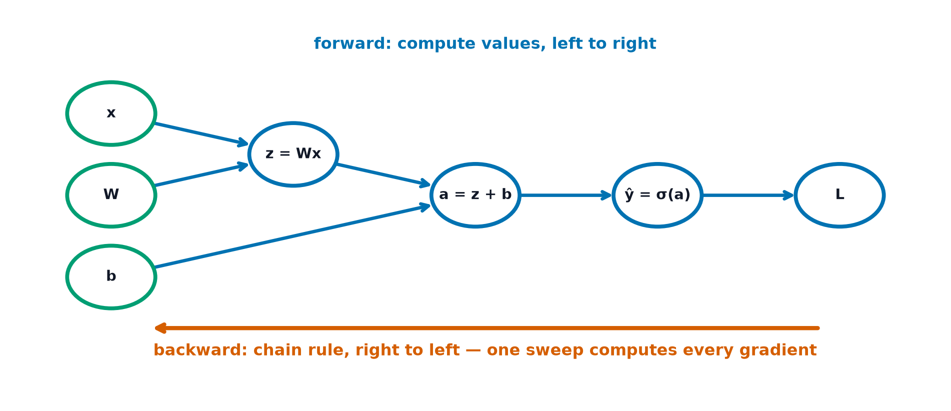
Writing the forward pass as a graph of primitive operations is what makes automatic differentiation mechanical rather than clever.

The forward pass computes values left to right; the backward pass applies the chain rule right to left. Every framework builds this graph so it can walk it backwards automatically.

Layer as affine transform plus activation

Each layer computes:

$$z^{[l]} = W^{[l]} a^{[l-1]} + b^{[l]}, \qquad a^{[l]} = g(z^{[l]})$$

An affine (linear-plus-offset) transform, then a non-linearity (Activation Functions) applied elementwise.

The full forward pass for an L-layer net

Starting from $a^{[0]} = x$ (the input), apply the layer equation above repeatedly for $l = 1, \ldots, L$, with $a^{[L]}$ the network's final output.

Shape bookkeeping

Quantity	Shape
$a^{[l-1]}$	$(n^{[l-1]}, )$ per example, or $(batch, n^{[l-1]})$ for a batch
$W^{[l]}$	$(n^{[l]}, n^{[l-1]})$
$b^{[l]}$	$(n^{[l]}, )$
$z^{[l]}, a^{[l]}$	$(n^{[l]}, )$ per example

Tracking these shapes explicitly at every layer is the single most useful habit for avoiding the broadcasting bugs introduced in Linear Algebra.

Batching, and why the batch dimension comes first

Processing examples one at a time wastes the parallel hardware GPUs and vectorised CPU operations are built for. Stacking $B$ examples into a single $(B, n^{[l-1]})$ matrix lets one matrix multiplication compute all $B$ forward passes simultaneously. The convention of putting the batch dimension first ((batch, features) rather than (features, batch)) is nearly universal across frameworks, though the underlying math is identical either way.

Symbol	Meaning
$z^{[l]}$	pre-activation (linear output) of layer $l$
$a^{[l]}$	post-activation output of layer $l$
$n^{[l]}$	number of units in layer $l$
$B$	batch size

The computational graph

Represent the forward pass as a directed graph: nodes are operations (matrix multiply, add, activation), edges are the tensors flowing between them. This is not a metaphor — frameworks like PyTorch build this exact graph at runtime as operations execute, and Backpropagation is simply traversing this graph in reverse.

Static vs. dynamic graphs

Static graphs (TensorFlow 1.x's original design) are built once, ahead of time, then executed repeatedly — allows aggressive optimisation but makes debugging and variable-length inputs awkward. Dynamic graphs (PyTorch, and now TensorFlow's default eager mode) are rebuilt on every forward pass, exactly following the Python control flow that ran — easier to debug (a stack trace points at real Python code) and naturally handles variable-length or conditional computation, at some historical optimisation cost that modern JIT compilers have largely closed.

Memory: what must be cached for the backward pass

Computing $\partial L / \partial W^{[l]}$ during backpropagation requires $a^{[l-1]}$ (from the forward pass) — so every intermediate activation must be kept in memory until its corresponding backward computation runs. This is exactly what GPU Training and Mixed Precision's gradient checkpointing trades away (recomputing instead of storing) when memory is the bottleneck.

Code: a forward pass with explicit shape assertions

forward_pass_demo.py

import numpy as np

def sigmoid(z):
    return 1 / (1 + np.exp(-z))

def forward_pass(x, layer_sizes, weights, biases, verbose=True):
    a = x
    if verbose:
        print(f"input shape: {a.shape}")
    for l, (W, b) in enumerate(zip(weights, biases)):
        z = a @ W + b
        assert z.shape == (a.shape[0], W.shape[1]), f"shape mismatch at layer {l}"
        a = sigmoid(z)
        if verbose:
            print(f"layer {l}: W{W.shape} -> z{z.shape} -> a{a.shape}")
    return a

rng = np.random.default_rng(0)
layer_sizes = [10, 32, 16, 1]  # input dim 10, two hidden layers, scalar output
batch_size = 8

weights = [rng.normal(scale=0.1, size=(layer_sizes[i], layer_sizes[i+1])) for i in range(len(layer_sizes)-1)]
biases = [np.zeros(layer_sizes[i+1]) for i in range(len(layer_sizes)-1)]

X = rng.normal(size=(batch_size, layer_sizes[0]))
output = forward_pass(X, layer_sizes, weights, biases)
print("final output shape:", output.shape)

# --- A deliberate shape mismatch, caught loudly ---
try:
    bad_weights = weights.copy()
    bad_weights[1] = rng.normal(size=(999, layer_sizes[2] + 1))  # wrong input dim
    forward_pass(X, layer_sizes, bad_weights, biases, verbose=False)
except (ValueError, AssertionError) as e:
    print(f"caught the expected shape error: {e}")

See also

• Backpropagation — differentiating this exact graph, edge by edge, in reverse.
• Linear Algebra — the matrix shapes and operations this forward pass is built from.