From Perceptron to MLP

In 1958, Frank Rosenblatt built a model that could learn simple logical patterns from data — and in 1969, Minsky and Papert proved it could never learn XOR, a result that froze neural network research for over a decade. The fix, once found, was a single conceptual change: stack more than one layer, with something non-linear between them.

Key idea

A single linear unit can only draw a straight boundary; stacking units with a non-linearity between them removes that ceiling entirely.

AND and OR need one line; XOR needs two. A single perceptron can only draw one, which is the limitation that stalled neural networks for years — and the reason a hidden layer exists.

The biological analogy, and how far it goes

The perceptron was loosely inspired by a biological neuron — inputs (dendrites) weighted and summed, compared against a threshold, producing an output (axon firing or not). The analogy is useful for intuition and stops there: real neurons involve timing, chemistry, and dynamics that this simplified model doesn't attempt to capture.

The perceptron: weights, bias, step activation

$$\hat y = \begin{cases} 1 & \text{if } w^\top x + b \ge 0 \\ 0 & \text{otherwise} \end{cases}$$

A weighted sum of inputs, compared against zero (the bias shifts where that comparison happens).

The perceptron learning rule

For each misclassified example, nudge the weights toward correcting it:

$$w \leftarrow w + \eta (y - \hat y) x$$

Guaranteed to converge to a perfect separator in finitely many steps — but only if the data is actually linearly separable.

What it can learn: AND, OR

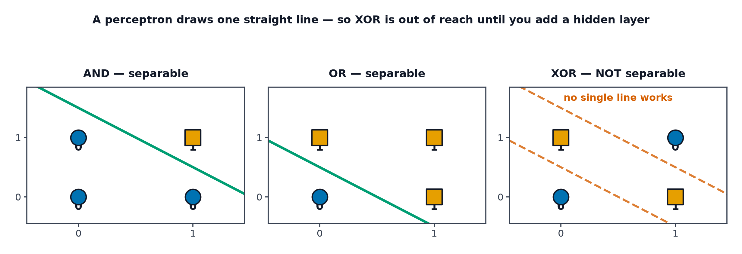
Both AND and OR are linearly separable — a single straight line divides the true outputs from the false ones in input space, so a perceptron can represent both.

The XOR problem, shown geometrically

XOR outputs true for $(0,1)$ and $(1,0)$, false for $(0,0)$ and $(1,1)$ — plot these four points and no single straight line separates the true pair from the false pair. XOR is not linearly separable, and a perceptron, being fundamentally a linear classifier, cannot represent it, no matter how the weights are set.

The 1969 winter and what it was really about

Minsky and Papert's proof that perceptrons cannot solve XOR was mathematically narrow (about single-layer perceptrons specifically) but was widely read as damning neural networks as a whole, contributing to a long funding and research drought. The irony: the fix (stacking layers) was already conceptually available, but the practical training algorithm for multi-layer networks (Backpropagation) wasn't popularised until the mid-1980s.

Stacking layers

$$h = g_1(W_1 x + b_1), \qquad \hat y = g_2(W_2 h + b_2)$$

A second layer, applied to the output of the first.

Why a stack of linear layers is still linear

If $g_1$ is the identity (no non-linearity), then:

$$\hat y = W_2(W_1 x + b_1) + b_2 = (W_2 W_1)x + (W_2 b_1 + b_2) = W' x + b'$$

Two linear layers compose into a single equivalent linear layer — depth buys nothing at all without a non-linearity between the layers. This is why "the non-linearity" gets its own emphasis: it's the only thing that makes stacking layers meaningfully more expressive than a single layer.

Symbol	Meaning
$W_1, W_2$	weight matrices of the two layers
$g_1$	the non-linear activation between layers, breaking the collapse
$h$	the hidden layer's activations

The non-linearity as the load-bearing component

Once $g_1$ is a genuine non-linearity (sigmoid, ReLU, etc. — Activation Functions), the collapse argument above no longer applies, and the two-layer network can represent functions a single linear layer cannot — including XOR.

The MLP

A multi-layer perceptron stacks several such layers: input, one or more hidden layers (each with a non-linearity), output. Despite the name, it's not perceptrons stacked — each unit computes a smooth (not step-function) transformation, trained by gradient descent rather than the perceptron rule.

Universal approximation theorem, stated honestly

A sufficiently wide single-hidden-layer network can approximate any continuous function on a bounded domain to arbitrary precision. This is an existence result, not a learnability or efficiency one: it says such a network exists, not that gradient descent will find it, and not that a shallow wide network is the most parameter-efficient way to represent the function — in practice, deeper (not just wider) networks tend to represent complex functions far more compactly.

Code: perceptron failing XOR, then a 2-layer network solving it

perceptron_to_mlp_demo.py

import numpy as np
import matplotlib.pyplot as plt

X_and = np.array([[0,0],[0,1],[1,0],[1,1]])
y_and = np.array([0,0,0,1])
X_xor = np.array([[0,0],[0,1],[1,0],[1,1]])
y_xor = np.array([0,1,1,0])

def perceptron_fit(X, y, lr=0.1, epochs=20):
    w, b = np.zeros(X.shape[1]), 0.0
    for _ in range(epochs):
        for xi, yi in zip(X, y):
            pred = int(w @ xi + b >= 0)
            w += lr * (yi - pred) * xi
            b += lr * (yi - pred)
    return w, b

w_and, b_and = perceptron_fit(X_and, y_and)
preds_and = [(w_and @ x + b_and >= 0) for x in X_and]
print("perceptron on AND:", preds_and, " target:", y_and.tolist(), " <- solves it")

w_xor, b_xor = perceptron_fit(X_xor, y_xor, epochs=100)
preds_xor = [int(w_xor @ x + b_xor >= 0) for x in X_xor]
print("perceptron on XOR:", preds_xor, " target:", y_xor.tolist(), " <- fails, no line separates XOR")

# --- A hand-built 2-layer network with a non-linearity, solving XOR ---
def sigmoid(z): return 1 / (1 + np.exp(-z))

rng = np.random.default_rng(0)
W1, b1 = rng.normal(size=(2, 4)), np.zeros(4)
W2, b2 = rng.normal(size=(4, 1)), np.zeros(1)
X, y = X_xor.astype(float), y_xor.reshape(-1, 1).astype(float)

for step in range(20000):
    h = sigmoid(X @ W1 + b1)
    out = sigmoid(h @ W2 + b2)
    d_out = (out - y) * out * (1 - out)
    d_h = (d_out @ W2.T) * h * (1 - h)
    W2 -= 0.5 * h.T @ d_out; b2 -= 0.5 * d_out.sum(0)
    W1 -= 0.5 * X.T @ d_h; b1 -= 0.5 * d_h.sum(0)

final_preds = (sigmoid(sigmoid(X @ W1 + b1) @ W2 + b2) >= 0.5).astype(int).ravel()
print("2-layer network on XOR:", final_preds.tolist(), " target:", y_xor.tolist(), " <- solves it")

The perceptron should visibly fail to converge on XOR (its predictions won't match the targets no matter how many epochs run), while the two-layer network with a sigmoid non-linearity solves it exactly — direct, runnable confirmation of the collapse argument above.

See also

• Activation Functions — the non-linearity that makes depth meaningful.
• Backpropagation — the training algorithm that made multi-layer networks practical.