Learning Rate Schedules

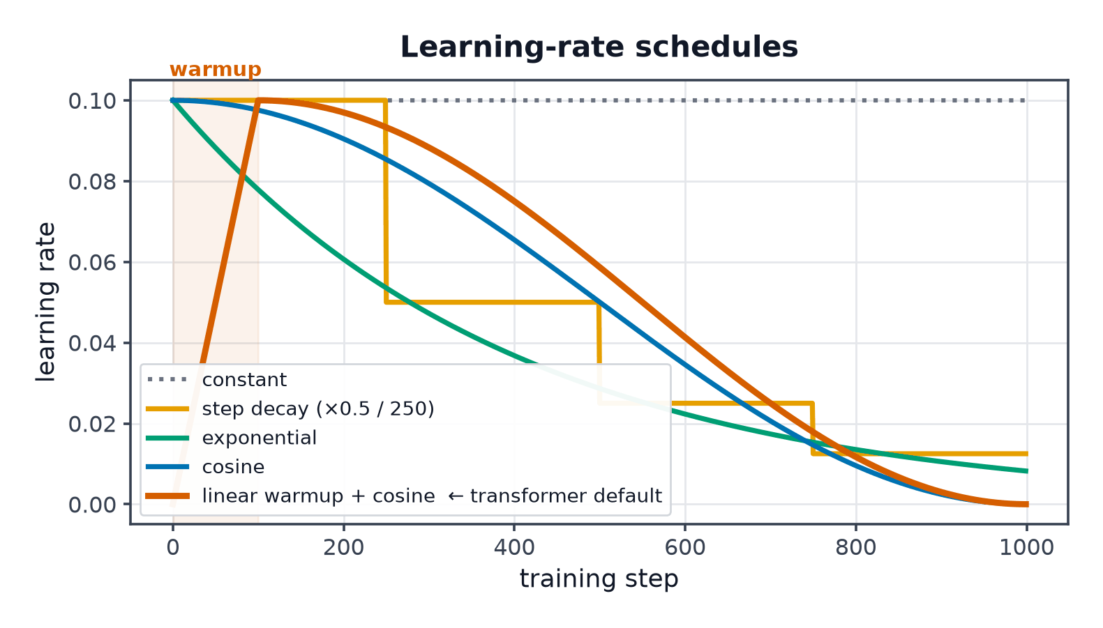
The learning rate is the single hyperparameter that most determines whether training works at all, and holding it fixed for the entire run is rarely the best choice. Every schedule on this page is a variation of the same idea: large steps early, when you're far from a good solution and want to explore quickly, small steps late, when you're close and want to settle precisely.

Key idea

Large steps early to explore, small steps late to settle — every schedule is a way of saying that.

Constant, step, exponential and cosine learning-rate schedules, plus linear warmup followed by cosine decay — Warmup plus cosine decay is the transformer default. The warmup exists because early gradients are large and poorly conditioned — starting at full rate can move the weights somewhere training never recovers from.

The learning rate as the dominant hyperparameter

Too high and training diverges outright; too low and training crawls, or gets stuck in a shallow local structure it could have escaped with a larger step. Nearly every other hyperparameter matters less than getting this one into a reasonable range first.

The LR range test for finding a starting value

Run a short training pass, increasing the learning rate exponentially from a tiny value to a large one over a few hundred steps, plotting loss against learning rate. The loss typically decreases, reaches a minimum, then rises sharply as the rate becomes too large — a good starting learning rate is usually an order of magnitude below where the loss starts rising.

Step decay

Reduce the learning rate by a fixed factor at fixed intervals (e.g. halve every 30 epochs) — simple, interpretable, requires manually choosing the decay points.

Exponential decay

\eta_t = \eta_0 \cdot \gamma^t

Smooth, continuous decay rather than step decay's discrete jumps — no manually-chosen decay points, but the decay rate $\gamma$ itself needs tuning.

Cosine annealing

\eta_t = \eta_{\min} + \frac{1}{2}(\eta_{\max} - \eta_{\min})\left(1 + \cos\left(\frac{t}{T}\pi\right)\right)

Smoothly decreases the learning rate following a cosine curve from $\eta_{\max}$ down to $\eta_{\min}$ over $T$ total steps — the most common single-cycle schedule in modern training, since it decays slowly at first (when large steps are still useful) and increasingly quickly as $t \to T$ (settling precisely at the end).

Symbol	Meaning
$\eta_0, \eta_{\max}, \eta_{\min}$	initial/maximum/minimum learning rate
$\gamma$	exponential decay factor
$T$	total number of steps in the schedule (or one cycle of it)

Warmup, and why transformers cannot train without it

Start the learning rate at (or near) zero and linearly ramp it up over the first few hundred/thousand steps before applying the main decay schedule. Without warmup, transformers (Transformer Architecture) frequently diverge in the very first steps — the Adam optimiser's early-step variance estimates are unreliable before enough gradient history has accumulated (the exact bias the correction terms in Optimizers address, but imperfectly at extremely small $t$ ), and a large learning rate applied to those unreliable estimates produces unstable early updates.

Warm restarts (SGDR)

Periodically reset the learning rate back up to $\eta_{\max}$ and run another cosine decay cycle — the idea being that each "restart" lets the optimiser escape a sharp local minimum and potentially settle into a broader, better-generalising one on the next cycle.

One-cycle

Ramp the learning rate up from a low value to a high peak over the first phase of training, then back down to a very low value over the remainder — combines warmup and decay into a single deliberate cycle, and has been shown empirically to allow faster overall convergence than a monotonic schedule in many settings.

Plateau-triggered reduction

Monitor validation loss; reduce the learning rate by a factor whenever it stops improving for a set number of epochs (ReduceLROnPlateau) — adaptive to the actual training dynamics rather than following a fixed schedule decided in advance.

Per-layer and discriminative learning rates for fine-tuning

When fine-tuning a pretrained model (Finetuning and Instruction Tuning), it's common to use a smaller learning rate for early (pretrained, already well-tuned) layers and a larger one for later or newly-added layers, since the early layers need only small adjustments while later/new layers need to learn more from scratch.

Reading a loss curve to diagnose the learning rate

Symptom	Diagnosis
Loss decreases very slowly, smoothly	LR too low
Loss decreases quickly then plateaus early, above where it should	LR too low, or needs decay
Loss oscillates wildly, doesn't consistently decrease	LR too high
Loss diverges (grows without bound)	LR far too high
Loss decreases well initially, degrades later	needs more data, or LR should have decayed by that point

Schedule selection table

Regime	Reach for
Training from scratch, standard setting	cosine annealing, possibly with warmup
Training a transformer	warmup + cosine or inverse-square-root decay
Fine-tuning a pretrained model	small constant LR, or discriminative per-layer rates
Uncertain how long training will run	plateau-triggered reduction
Want fastest convergence with careful tuning	one-cycle

Code: plotting every schedule, then training runs compared

lr_schedules_demo.py
import numpy as np
import matplotlib.pyplot as plt

steps = np.arange(0, 1000)

def step_decay(t, eta0=0.1, drop=0.5, every=300): return eta0 * drop ** (t // every)
def exp_decay(t, eta0=0.1, gamma=0.995): return eta0 * gamma ** t
def cosine(t, eta_max=0.1, eta_min=0.001, T=1000): return eta_min + 0.5*(eta_max-eta_min)*(1+np.cos(t/T*np.pi))
def warmup_cosine(t, eta_max=0.1, eta_min=0.001, T=1000, warmup=100):
    if t < warmup: return eta_max * t / warmup
    return cosine(t - warmup, eta_max, eta_min, T - warmup)

fig, ax = plt.subplots(figsize=(8, 5))
for name, fn in [("step decay", step_decay), ("exponential", exp_decay),
                  ("cosine", cosine), ("warmup + cosine", warmup_cosine)]:
    ax.plot(steps, [fn(t) for t in steps], label=name)
ax.legend(); ax.set_xlabel("step"); ax.set_ylabel("learning rate")
plt.savefig("lr_schedules.png")

# --- Short training run: three fixed LRs plus a cosine schedule ---
rng = np.random.default_rng(0)
X = rng.normal(size=(200, 5)); true_w = rng.normal(size=5)
y = X @ true_w + rng.normal(scale=0.1, size=200)

def train(lr_fn, steps=300):
    w = np.zeros(5); losses = []
    for t in range(steps):
        lr = lr_fn(t) if callable(lr_fn) else lr_fn
        grad = 2 * X.T @ (X @ w - y) / len(y)
        w -= lr * grad
        losses.append(np.mean((X @ w - y) ** 2))
    return losses

fig, ax = plt.subplots()
for label, lr in [("lr=0.001 (too small)", 0.001), ("lr=0.05 (healthy fixed)", 0.05),
                    ("lr=0.3 (too large)", 0.3), ("cosine schedule", lambda t: cosine(t, 0.3, 0.001, 300))]:
    ax.plot(train(lr), label=label)
ax.set_yscale("log"); ax.legend()
plt.savefig("lr_training_comparison.png")

The learning rate as the dominant hyperparameter​

The LR range test for finding a starting value​

Step decay​

Exponential decay​

Cosine annealing​

Warmup, and why transformers cannot train without it​

Warm restarts (SGDR)​

One-cycle​

Plateau-triggered reduction​

Per-layer and discriminative learning rates for fine-tuning​

Reading a loss curve to diagnose the learning rate​

Schedule selection table​

Code: plotting every schedule, then training runs compared​

See also​