Model Capacity and Scaling

How big should the model be? The classical answer from Bias-Variance Tradeoff — bigger risks overfitting past some point — turns out to be incomplete for the over-parameterised networks that now dominate deep learning, where a second, deeper descent in test error can appear past the point where the classical U-curve says things should be getting worse.

Key idea

Capacity, data, and compute are jointly constrained — scaling one without the others buys nothing.

Loss falls as a power law in parameters, data and compute — straight lines on log–log axes. Each compute budget has its own optimal model size, which is the result Chinchilla made concrete.

Parameter count as a crude capacity proxy

More parameters generally means more representational capacity — but it's a crude proxy: architecture matters enormously (a well-designed 10M-parameter CNN can outperform a poorly-designed 50M-parameter one), and not every parameter contributes equally to a model's effective expressiveness.

Depth vs. width

Depth (more layers) tends to let a network compose increasingly abstract features, one layer building on the last. Width (more units per layer) increases capacity at a single level of abstraction without adding compositional depth. Skip Connections and Depth is precisely what made depth a practically usable lever rather than a purely theoretical one.

The classical U-curve and where it comes from

Bias-Variance Tradeoff's story: as capacity grows, training error monotonically falls, but test error falls, then rises again past the point where the model has enough capacity to start memorising noise in the training set — the classical prescription is to stop capacity right around that turning point.

Double descent

Modern over-parameterised networks, pushed well past the point where they can perfectly fit (interpolate) the training data, often show test error rising near that interpolation threshold (as the classical story predicts) — and then descending a second time as capacity continues to grow further beyond it. The classical U-curve isn't wrong; it's the first half of a more complete picture that the field hadn't observed until models routinely had far more parameters than training examples.

Scaling laws

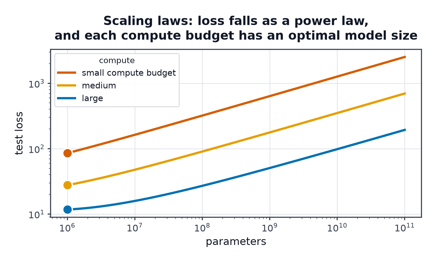
Empirically, loss on a well-defined task tends to follow a power-law relationship with the number of parameters $N$, the amount of training data $D$, and the compute budget $C$, each held roughly fixed while the other varies:

$$L(N) \approx \left(\frac{N_c}{N}\right)^\alpha$$

Symbol	Meaning
$L(N)$	achievable loss as a function of parameter count
$N_c$	a task-specific constant
$\alpha$	the power-law exponent, typically a small positive number
$C \approx 6ND$	the approximate compute cost (FLOPs) to train a model of size $N$ on $D$ tokens/examples

Compute-optimal training

Given a fixed compute budget $C$, there's a joint choice of model size $N$ and data size $D$ that minimises loss — and research into this trade (notably the "Chinchilla" scaling analysis) found that many earlier large models were substantially over-sized relative to the data they were trained on: for a fixed compute budget, a smaller model trained on proportionally more data often outperforms a larger model trained on less, a genuinely counter-intuitive finding at the time it was published, since "bigger model" had been the dominant lever pulled until then.

Emergent behaviour claims, and the honest caveats

Some capabilities have been reported to appear only above a certain model scale, seemingly discontinuously ("emergent abilities"). A meaningful fraction of these reported jumps have since been shown, in follow-up work, to be partly an artefact of the specific metric used (a metric with a hard pass/fail threshold can look like a sudden jump even when the underlying continuous quantity it's derived from was improving smoothly all along) — genuinely emergent, non-metric-artefact behaviour likely exists, but the claim deserves more scrutiny per instance than the phrase "emergent abilities" alone tends to receive.

The practical sizing procedure

Start small and cheap; identify empirically which of capacity, data, or compute is the binding constraint on your specific task and dataset (a learning curve that's still climbing steeply with more data suggests data is binding; one that's flat regardless of model size suggests capacity elsewhere in the pipeline, like feature quality, is binding); scale whichever lever the evidence points to, rather than defaulting to "bigger model" as the first move.

When scaling is the wrong answer

Scaling model size does nothing to fix mislabelled training data, a poorly chosen objective that doesn't actually reflect the real task, or a fundamentally missing feature/signal the model has no way to learn from — these are the more common actual bottlenecks in applied work, and no amount of additional capacity, data, or compute compensates for them.

Code: reproducible double descent, and a small scaling sweep

model_capacity_demo.py

import numpy as np
import matplotlib.pyplot as plt

# --- Double descent: random-feature regression, sweeping past the interpolation threshold ---
rng = np.random.default_rng(0)
n_train, n_test, d_input = 40, 200, 20

X_train = rng.normal(size=(n_train, d_input))
true_w = rng.normal(size=d_input)
y_train = X_train @ true_w + rng.normal(scale=1.0, size=n_train)
X_test = rng.normal(size=(n_test, d_input))
y_test = X_test @ true_w + rng.normal(scale=1.0, size=n_test)

feature_counts = list(range(2, 200, 4))
test_errors = []
for n_features in feature_counts:
    W_random = rng.normal(size=(d_input, n_features)) / np.sqrt(d_input)  # fixed random projection
    phi_train = np.maximum(0, X_train @ W_random)  # random ReLU features
    phi_test = np.maximum(0, X_test @ W_random)
    # minimum-norm solution (pseudo-inverse), the natural choice past the interpolation threshold
    w_fit = np.linalg.pinv(phi_train) @ y_train
    test_error = np.mean((phi_test @ w_fit - y_test) ** 2)
    test_errors.append(test_error)

fig, ax = plt.subplots()
ax.plot(feature_counts, test_errors)
ax.axvline(n_train, color="red", linestyle="--", label=f"interpolation threshold (n={n_train})")
ax.set_yscale("log"); ax.set_xlabel("number of random features"); ax.legend()
plt.savefig("double_descent.png")
print("test error near threshold vs far past it:",
      f"{test_errors[feature_counts.index(min(feature_counts, key=lambda x: abs(x-n_train)))]:.2f}",
      "vs", f"{test_errors[-1]:.2f}")

# --- Small scaling sweep: loss vs parameter count, log-log ---
import torch
import torch.nn as nn

X_t = torch.randn(500, 10)
y_t = (X_t.sum(dim=1, keepdim=True) + 0.3 * torch.randn(500, 1))

widths = [4, 16, 64, 256]
final_losses = []
for width in widths:
    torch.manual_seed(0)
    model = nn.Sequential(nn.Linear(10, width), nn.ReLU(), nn.Linear(width, 1))
    optimizer = torch.optim.Adam(model.parameters(), lr=0.01)
    for _ in range(500):
        optimizer.zero_grad()
        loss = ((model(X_t) - y_t) ** 2).mean()
        loss.backward()
        optimizer.step()
    final_losses.append(loss.item())
    n_params = sum(p.numel() for p in model.parameters())
    print(f"width={width:4d} ({n_params:5d} params): final loss={loss.item():.4f}")

See also

• Bias-Variance Tradeoff — the classical theory double descent extends past its original boundary.
• Skip Connections and Depth — the architectural change that made scaling depth practically feasible.