Normalization Layers

Networks deeper than twenty or so layers were, for years, essentially untrainable — every layer's input distribution kept shifting as the layers below it updated, forcing each layer to constantly re-adapt to a moving target. Batch normalisation, and the family of normalisation layers it started, fixed this directly by re-standardising activations at every layer, which is what let networks scale to hundreds of layers.

Key idea

Normalising activations inside the network keeps every layer's input distribution stable, which lets you use higher learning rates without divergence.

The only thing separating these four is which axes get averaged into one mean and variance. Batch norm reaches across the batch — which is why it misbehaves at batch size 1 and why transformers use layer norm instead.

The problem: distribution shift between layers

Without normalization the pre-activation distribution drifts and widens with depth. Keeping it centred is what allows a higher learning rate, which is where most of the speed-up actually comes from.

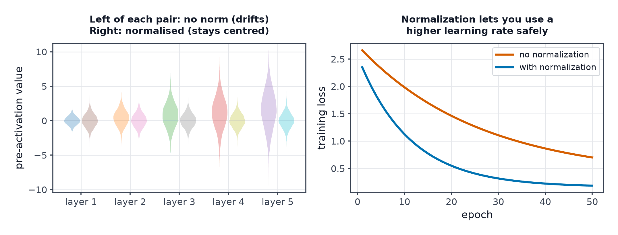
As training updates earlier layers' weights, the distribution of activations feeding into later layers keeps changing, layer by layer, step by step — every layer is perpetually adapting to a target that itself keeps moving, which slows convergence and makes high learning rates risky.

Batch normalisation: the algorithm

For a mini-batch, normalise each feature to zero mean, unit variance, then apply a learned scale and shift:

$$\hat x = \frac{x - \mu_B}{\sqrt{\sigma_B^2 + \epsilon}}, \qquad y = \gamma \hat x + \beta$$

Symbol	Meaning
$\mu_B, \sigma_B^2$	mean and variance computed across the current mini-batch
$\gamma, \beta$	learned scale and shift, one pair per feature
$\epsilon$	small constant preventing division by zero

Why γ and β exist

If BatchNorm only normalised (no $\gamma, \beta$), it would force every layer's output to have exactly zero mean and unit variance — but that's not always the ideal distribution for the following layer. $\gamma$ and $\beta$ let the network learn to undo the normalisation if that's actually better, restoring full representational flexibility on top of the stabilisation benefit.

Train vs. inference behaviour, and the running-statistics trap

During training, $\mu_B, \sigma_B^2$ are computed from the current mini-batch. At inference, batches may be size 1 or absent entirely, so BatchNorm instead uses a running average of $\mu_B, \sigma_B^2$ accumulated during training. The trap: forgetting to switch a model into evaluation mode (model.eval() in PyTorch) leaves BatchNorm using live batch statistics at inference time instead of the frozen running averages — a common, quiet bug covered further in Training Loop Anatomy.

Batch size dependence

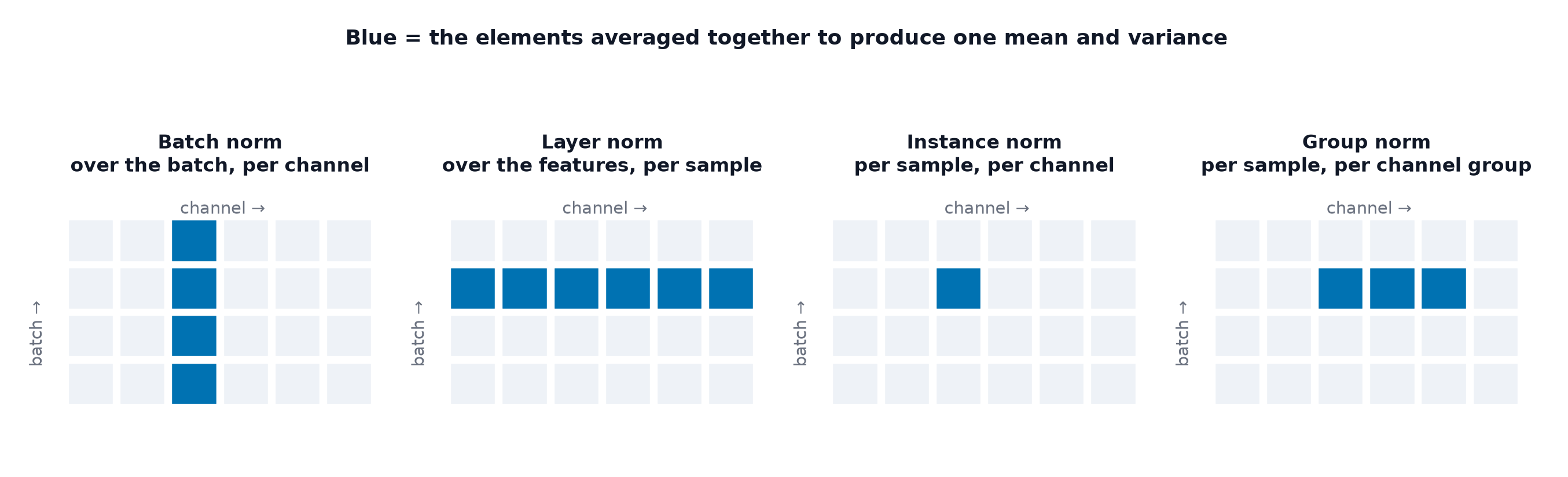
BatchNorm's statistics are only meaningful when computed over a reasonably-sized batch — at batch size 1, $\sigma_B^2$ is undefined (or zero), and BatchNorm effectively breaks. This dependency on batch size is BatchNorm's core limitation.

Layer normalisation

Instead of normalising across the batch dimension, LayerNorm normalises across the feature dimension, independently for each example:

$$\hat x_i = \frac{x_i - \mu_i}{\sqrt{\sigma_i^2 + \epsilon}}, \quad \text{where } \mu_i, \sigma_i^2 \text{ are computed over that example's features}$$

This has no batch-size dependency at all (each example is normalised independently), which is exactly why NLP and transformer architectures (Transformer Architecture) use LayerNorm almost universally — sequence lengths vary, batch sizes vary, and BatchNorm's batch-statistics dependency doesn't fit that setting well.

Instance and group normalisation

Instance normalisation: normalises per-example, per-channel (common in style-transfer vision models). Group normalisation: normalises per-example, over a group of channels — a middle ground between LayerNorm (all channels) and InstanceNorm (each channel alone), useful when batch sizes are too small for BatchNorm but full per-channel independence (InstanceNorm) is too aggressive.

RMSNorm

A simplified LayerNorm variant that skips mean-centring, normalising only by the root-mean-square:

$$\hat x_i = \frac{x_i}{\sqrt{\frac{1}{d}\sum_j x_{ij}^2 + \epsilon}}$$

Cheaper to compute than full LayerNorm, and used in several modern large language models with negligible quality difference observed.

Pre-norm vs. post-norm in transformers

Post-norm (the original transformer design): apply normalisation after the residual addition. Pre-norm: apply normalisation before each sub-layer, with the residual connection bypassing the normalisation entirely. Pre-norm produces a cleaner, more direct gradient path through the residual stream (see Skip Connections and Depth), and has become the standard choice for training very deep transformers — post-norm can require careful learning-rate warmup to avoid early divergence that pre-norm is substantially more robust to.

The "internal covariate shift" explanation, and the evidence against it

BatchNorm's original paper attributed its benefit to reducing "internal covariate shift" (the layer-to-layer distribution drift described above). Later empirical work found evidence that BatchNorm's main benefit may instead come from smoothing the loss landscape — making the gradient more predictable and less erratic — rather than the originally-proposed mechanism. The debate is not fully settled; the practical benefit (BatchNorm reliably helps) is far better established than the theoretical explanation for why.

Selection table

Architecture	Default normalisation
CNNs, large batch size	BatchNorm
CNNs, small batch size	GroupNorm
Transformers, RNNs, variable-length sequences	LayerNorm (or RMSNorm)
Style transfer / generative vision	InstanceNorm

Code: BatchNorm train/inference modes, and a deep network with/without it

normalization_demo.py

import numpy as np

class BatchNorm:
    def __init__(self, n_features, momentum=0.9, eps=1e-5):
        self.gamma, self.beta = np.ones(n_features), np.zeros(n_features)
        self.running_mean, self.running_var = np.zeros(n_features), np.ones(n_features)
        self.momentum, self.eps = momentum, eps

    def forward(self, x, training=True):
        if training:
            mu, var = x.mean(axis=0), x.var(axis=0)
            self.running_mean = self.momentum * self.running_mean + (1-self.momentum) * mu
            self.running_var = self.momentum * self.running_var + (1-self.momentum) * var
        else:
            mu, var = self.running_mean, self.running_var  # frozen statistics
        x_hat = (x - mu) / np.sqrt(var + self.eps)
        return self.gamma * x_hat + self.beta

rng = np.random.default_rng(0)
bn = BatchNorm(n_features=5)
for _ in range(50):
    bn.forward(rng.normal(loc=3, scale=2, size=(32, 5)), training=True)

test_batch = rng.normal(loc=3, scale=2, size=(1, 5))  # batch size 1 - only survives via running stats
out_correct = bn.forward(test_batch, training=False)
print("inference mode (uses running stats, batch_size=1 safe):", out_correct.round(3))

# --- Deep network: with vs without normalisation, aggressive learning rate ---
def relu(z): return np.maximum(0, z)

def train_deep_net(use_bn, lr=1.0, depth=15, width=50, steps=100):
    rng2 = np.random.default_rng(1)
    Ws = [rng2.normal(scale=np.sqrt(2/width), size=(width, width)) for _ in range(depth)]
    X = rng2.normal(size=(64, width))
    losses = []
    for step in range(steps):
        a = X
        for W in Ws:
            z = a @ W
            if use_bn:
                z = (z - z.mean(0)) / np.sqrt(z.var(0) + 1e-5)  # simplified BN forward only
            a = relu(z)
        loss = np.mean(a ** 2)
        losses.append(loss if np.isfinite(loss) else np.nan)
    return losses

losses_with_bn = train_deep_net(use_bn=True)
losses_without_bn = train_deep_net(use_bn=False)
print(f"\nfinal activation magnitude WITH normalisation:    {losses_with_bn[-1]:.4f}")
print(f"final activation magnitude WITHOUT normalisation: {losses_without_bn[-1]}")

See also

• Weight Initialization — the initial-variance concern normalisation layers substantially (but not entirely) relax.
• Skip Connections and Depth — pre-norm placement's relationship to residual gradient flow.