Optimizers

Plain gradient descent takes the same fixed-size step in every direction, every time, regardless of the loss surface's shape. Everything covered on this page is a way of using information from past gradients to take smarter steps — and by the mid-2010s, one method (Adam) had absorbed most of these ideas and become the default nearly everyone reaches for first.

Key idea

Modern optimisers differ in how they estimate the direction (momentum) and how they scale each coordinate (adaptive learning rates).

A ravine — steep across, shallow along — is the surface that separates the optimizers. At a well-tuned rate SGD still flips sign on all 60 steps and stops short; momentum reaches the minimum with 13 oscillations. These paths are simulated, not sketched.

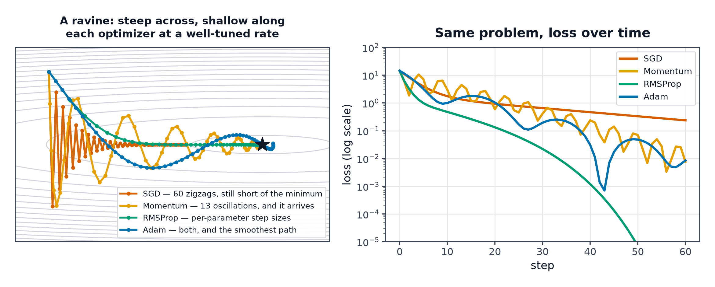
SGD recap and its problems

Plain Gradient Descent — $w \leftarrow w - \eta \nabla L(w)$ — struggles with three things: narrow ravines (it oscillates across the narrow direction while barely progressing along the long direction), noisy gradients (mini-batch estimates jitter around the true gradient), and a single learning rate applied identically to every parameter regardless of how differently-scaled their gradients are.

Momentum

$$v \leftarrow \beta v + \nabla L(w), \qquad w \leftarrow w - \eta v$$

Accumulates a running average of past gradients — consistent downhill directions build up speed, oscillating directions partially cancel. The heavy-ball analogy: a ball rolling downhill accelerates on a consistent slope and doesn't reverse instantly in a narrow ravine, unlike a memoryless point mass.

Nesterov accelerated gradient

A refinement: compute the gradient not at the current position, but at the position momentum is about to carry you to — a "look-ahead" correction that anticipates and partially corrects for overshoot, generally converging slightly faster than plain momentum.

AdaGrad

$$w \leftarrow w - \frac{\eta}{\sqrt{G + \epsilon}} \nabla L(w), \qquad G \leftarrow G + \nabla L(w)^2$$

Divides each parameter's learning rate by the square root of its accumulated squared gradient history — parameters with consistently large gradients get their effective learning rate shrunk, parameters with small gradients keep a relatively larger one. The problem: $G$ only ever grows, so the effective learning rate monotonically shrinks toward zero over a long training run, eventually halting learning entirely.

RMSProp

Fixes AdaGrad's decay problem by using an exponentially decaying average of squared gradients instead of an ever-growing sum:

$$G \leftarrow \gamma G + (1-\gamma)\nabla L(w)^2, \qquad w \leftarrow w - \frac{\eta}{\sqrt{G+\epsilon}}\nabla L(w)$$

Recent gradients matter more than ancient ones, so the effective learning rate can recover rather than only ever shrinking.

Adam: momentum plus RMSProp, with bias correction

$$m \leftarrow \beta_1 m + (1-\beta_1)\nabla L(w), \qquad v \leftarrow \beta_2 v + (1-\beta_2)\nabla L(w)^2$$ $$\hat m = \frac{m}{1-\beta_1^t}, \qquad \hat v = \frac{v}{1-\beta_2^t}, \qquad w \leftarrow w - \frac{\eta}{\sqrt{\hat v}+\epsilon}\hat m$$

Combines momentum's direction-smoothing ($m$) with RMSProp's per-parameter scaling ($v$).

Why bias correction exists, derived

$m$ and $v$ are initialised to zero, and the exponential moving average formula is biased toward zero especially in early steps (at $t=1$, $m = (1-\beta_1)\nabla L$, far smaller than the true gradient magnitude, since it started from zero). Dividing by $(1-\beta_1^t)$ and $(1-\beta_2^t)$ exactly corrects this early-step bias — as $t$ grows large, both correction factors approach 1 and have negligible effect, but they matter substantially in the first few steps.

Symbol	Meaning
$m, v$	first and second moment estimates (mean and uncentred variance of gradients)
$\beta_1, \beta_2$	decay rates for the two moment estimates (typically 0.9, 0.999)
$\hat m, \hat v$	bias-corrected moment estimates

AdamW and the weight-decay/L2 distinction

In plain Adam, adding an L2 penalty to the loss (as in Overfitting and Regularization) interacts oddly with the adaptive per-parameter scaling — the effective weight-decay strength ends up different for every parameter, since it's divided by $\sqrt{\hat v}$ along with the gradient. AdamW decouples weight decay from the gradient-based update entirely, applying it as a direct, uniform shrinkage of the weights independent of the adaptive scaling — now the standard choice for training transformers and most modern architectures.

Comparison table

	Memory (per param)	Key hyperparameters	Typical use
SGD+momentum	1x ($v$)	$\eta$, $\beta$	vision models, when tuned carefully
RMSProp	1x ($G$)	$\eta$, $\gamma$	RNNs, historically
Adam / AdamW	2x ($m$, $v$)	$\eta$, $\beta_1$, $\beta_2$	default for transformers, most modern work

The honest state of play

Despite Adam's popularity, well-tuned SGD with momentum still wins on some vision benchmarks (notably some ImageNet-scale CNN training), generalising slightly better in certain regimes — the practical advice is that Adam/AdamW is the safer, faster-converging default with minimal tuning, while SGD+momentum remains worth trying when squeezing out the last bit of generalisation performance matters and there's compute budget for extra tuning.

Code: SGD, momentum, RMSProp, Adam from scratch on a shared loss surface

optimizers_demo.py

import numpy as np
import matplotlib.pyplot as plt

def loss(w):
    return 0.1 * w[0]**2 + 2.0 * w[1]**2  # an elongated ravine

def grad(w):
    return np.array([0.2 * w[0], 4.0 * w[1]])

def run_sgd(lr=0.3, steps=60):
    w = np.array([-4.0, 1.0]); path = [w.copy()]
    for _ in range(steps):
        w = w - lr * grad(w); path.append(w.copy())
    return np.array(path)

def run_momentum(lr=0.3, beta=0.9, steps=60):
    w = np.array([-4.0, 1.0]); v = np.zeros(2); path = [w.copy()]
    for _ in range(steps):
        v = beta * v + grad(w); w = w - lr * v; path.append(w.copy())
    return np.array(path)

def run_rmsprop(lr=0.3, gamma=0.9, eps=1e-8, steps=60):
    w = np.array([-4.0, 1.0]); G = np.zeros(2); path = [w.copy()]
    for _ in range(steps):
        g = grad(w); G = gamma * G + (1-gamma) * g**2
        w = w - lr * g / (np.sqrt(G) + eps); path.append(w.copy())
    return np.array(path)

def run_adam(lr=0.3, b1=0.9, b2=0.999, eps=1e-8, steps=60):
    w = np.array([-4.0, 1.0]); m = np.zeros(2); v = np.zeros(2); path = [w.copy()]
    for t in range(1, steps+1):
        g = grad(w)
        m = b1*m + (1-b1)*g; v = b2*v + (1-b2)*g**2
        m_hat = m/(1-b1**t); v_hat = v/(1-b2**t)
        w = w - lr * m_hat / (np.sqrt(v_hat) + eps); path.append(w.copy())
    return np.array(path)

fig, ax = plt.subplots(figsize=(8, 6))
xx, yy = np.meshgrid(np.linspace(-5, 1, 100), np.linspace(-2, 2, 100))
zz = 0.1 * xx**2 + 2.0 * yy**2
ax.contour(xx, yy, zz, levels=20)
for name, path in [("SGD", run_sgd()), ("Momentum", run_momentum()), ("RMSProp", run_rmsprop()), ("Adam", run_adam())]:
    ax.plot(path[:, 0], path[:, 1], marker=".", label=name)
ax.legend()
plt.savefig("optimizer_trajectories.png")

Plain SGD should visibly zigzag across the narrow (steep) direction while crawling slowly along the shallow direction; momentum and Adam should reach the minimum in noticeably fewer, straighter steps.

See also

• Gradient Descent — the base algorithm every optimiser here extends.
• Learning Rate Schedules — varying $\eta$ itself over the course of training.