Regularization in Deep Nets

A modern network routinely has more parameters than training examples — by classical statistical intuition, this should guarantee catastrophic overfitting. It usually doesn't, and the regularisation techniques on this page are less about shrinking weights (as in Overfitting and Regularization's classical L1/L2 story) and more about injecting noise or stopping early.

Key idea

Deep-net regularisation is mostly about injecting noise or stopping early, not about shrinking weights.

Why over-parameterised networks generalise at all

This remains an active research question without a fully settled theoretical answer. Empirically, gradient descent with common initialisation schemes tends to find comparatively "simple" solutions among the many that fit the training data perfectly — a bias toward smooth, low-complexity functions that isn't fully explained by classical statistical learning theory, and is closely related to the double descent phenomenon.

Weight decay and its relationship to L2

Weight decay directly shrinks weights each step: $w \leftarrow w - \eta(\nabla L + \lambda w)$. For plain SGD, this is mathematically identical to adding an L2 penalty to the loss. For Adam, the two are not identical (as covered in Optimizers's AdamW discussion) — this is exactly the distinction that motivated AdamW's decoupled implementation.

Dropout: the algorithm

Dropout samples a different subnetwork every batch, so no unit can rely on any specific other unit being present. At test time the full network is used with activations scaled to match the training-time expectation.

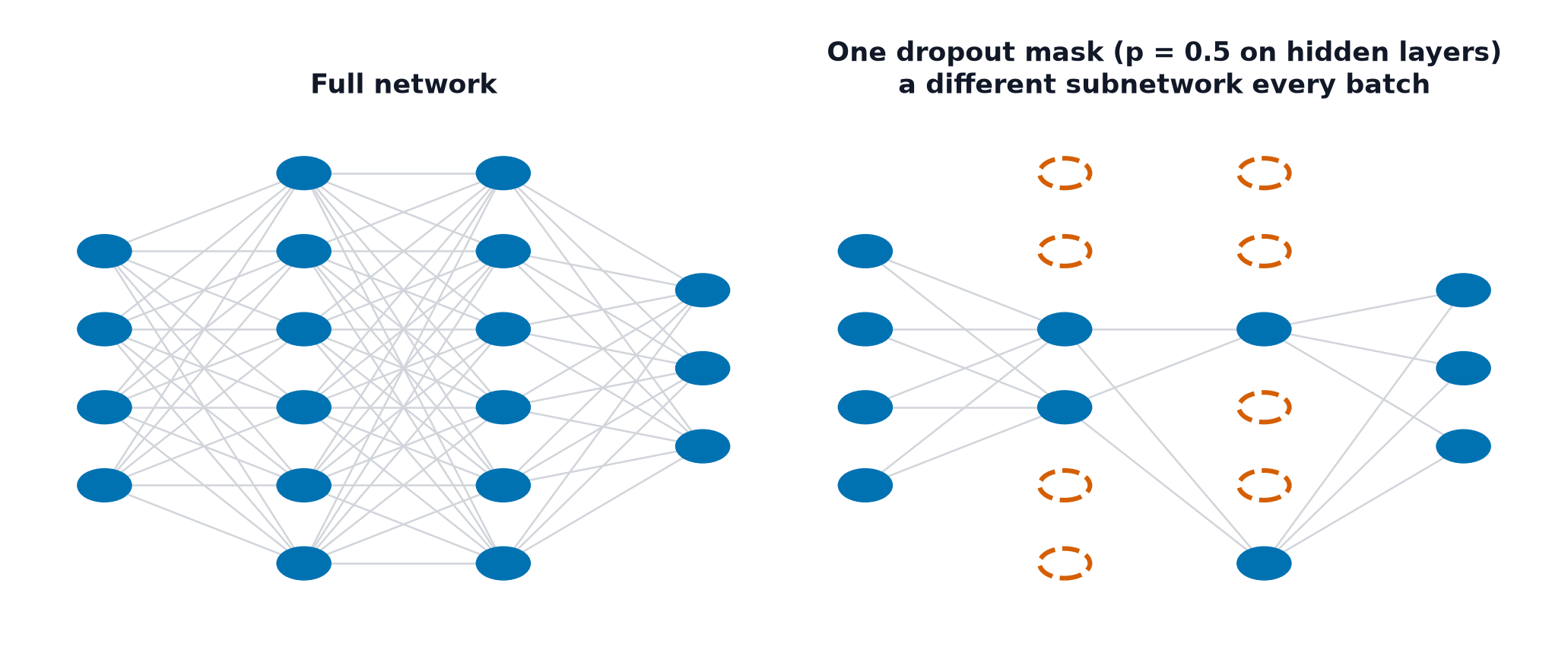
During training, randomly zero out each unit's activation with probability $p$ (independently, per unit, per forward pass):

$$\tilde a = a \odot m, \quad m_i \sim \text{Bernoulli}(1-p)$$

The ensemble interpretation

Each forward pass with a different random dropout mask effectively trains a different, smaller sub-network sharing the full network's weights. Training with dropout is loosely equivalent to training an enormous ensemble of these overlapping sub-networks simultaneously, and inference approximates averaging their predictions — an ensemble effect obtained without the cost of training or storing separate models.

Inverted dropout at inference

$$\tilde a_{\text{train}} = \frac{a \odot m}{1-p}$$

Dividing by $(1-p)$ during training (rather than scaling at inference) keeps the expected activation magnitude unchanged between train and inference time, so inference requires no special-case scaling — just skip the dropout mask entirely and use the raw activations.

Symbol	Meaning
$p$	dropout probability — fraction of units zeroed each pass
$m$	the random binary dropout mask, resampled every forward pass

Where dropout helps, and where it now mostly doesn't

Dropout was essential in early large fully-connected and convolutional networks. In modern CNNs trained with Normalization Layers (particularly BatchNorm), dropout's benefit is often small or negligible — BatchNorm's own noise (from mini-batch statistics) already provides a related regularising effect, and the two can interact poorly when combined carelessly. Dropout remains widely used in transformer feed-forward and attention blocks, and in fully-connected layers generally.

Early stopping as implicit regularisation

Monitor validation loss; stop (or restore the best checkpoint) once it stops improving — from Overfitting and Regularization, applied here specifically to deep network training runs where a single training run can span many hours and checkpointing is standard practice regardless.

Data augmentation as the strongest lever

For image, audio, and text data, synthetic transformations that preserve the label (crops, flips, noise, paraphrasing) are frequently the single most effective regulariser available — see Data Augmentation for the vision-specific deep dive.

Label smoothing

Instead of training toward a hard one-hot target (probability 1 for the true class, 0 for all others), soften the target slightly: $(1-\epsilon)$ for the true class, $\epsilon/(K-1)$ spread across the rest. This discourages the network from becoming overconfident — a network trained on hard targets can push logits toward $\pm\infty$ to approach probability exactly 1, which label smoothing directly prevents by capping the achievable target probability below 1.

Mixup and cutmix, briefly

Mixup: train on linear interpolations of pairs of examples and their labels — $\tilde x = \lambda x_1 + (1-\lambda)x_2$, $\tilde y = \lambda y_1 + (1-\lambda)y_2$. CutMix: paste a rectangular patch from one image onto another, mixing labels proportionally to the patch area. Both encourage smoother decision boundaries between classes by training on realistic interpolations rather than only pure examples.

Stochastic depth

For very deep residual networks, randomly skip entire residual blocks during training (using the identity path instead) — analogous to dropout, but at the level of whole layers rather than individual units, effectively training an ensemble of networks with varying depth.

Gradient clipping

Cap the gradient's norm (or individual values) before the optimiser step — this is a training-stability control rather than a generalisation regulariser, but it's grouped with these techniques since it's applied at the same point in the training loop; full treatment in Vanishing and Exploding Gradients.

Selection table

Symptom	Reach for
Fully-connected layers overfitting	dropout
CNN with BatchNorm already overfitting	data augmentation first, dropout second
Overconfident, poorly-calibrated predictions	label smoothing
Small dataset, image/audio/text	data augmentation, mixup/cutmix
Very deep residual network, slow/unstable training	stochastic depth
Loss occasionally spikes or diverges	gradient clipping

Code: inverted dropout from scratch, with vs. without on insufficient data

dropout_demo.py

import numpy as np

def relu(z): return np.maximum(0, z)

def dropout_forward(a, p, training):
    if not training:
        return a  # inference: no masking, no scaling needed (inverted dropout)
    mask = (np.random.rand(*a.shape) > p).astype(float)
    return (a * mask) / (1 - p)

rng = np.random.default_rng(0)
n_train, n_features = 30, 50  # deliberately few examples relative to features
X_train = rng.normal(size=(n_train, n_features))
true_w = rng.normal(size=n_features)
y_train = (X_train @ true_w > 0).astype(float).reshape(-1, 1)
X_test = rng.normal(size=(200, n_features))
y_test = (X_test @ true_w > 0).astype(float).reshape(-1, 1)

def train_net(use_dropout, p=0.5, hidden=100, steps=2000, lr=0.1):
    W1 = rng.normal(scale=0.1, size=(n_features, hidden)); b1 = np.zeros(hidden)
    W2 = rng.normal(scale=0.1, size=(hidden, 1)); b2 = np.zeros(1)
    for step in range(steps):
        h = relu(X_train @ W1 + b1)
        h_drop = dropout_forward(h, p, training=use_dropout)
        out = 1 / (1 + np.exp(-(h_drop @ W2 + b2)))
        d_out = out - y_train
        W2 -= lr * h_drop.T @ d_out / n_train; b2 -= lr * d_out.mean(0)
        d_h = (d_out @ W2.T) * (h > 0)
        W1 -= lr * X_train.T @ d_h / n_train; b1 -= lr * d_h.mean(0)
    def predict(X):
        h = relu(X @ W1 + b1)
        return (1 / (1 + np.exp(-(h @ W2 + b2))) > 0.5).astype(float)
    train_acc = (predict(X_train) == y_train).mean()
    test_acc = (predict(X_test) == y_test).mean()
    return train_acc, test_acc

for use_dropout in [False, True]:
    train_acc, test_acc = train_net(use_dropout)
    label = "WITH dropout" if use_dropout else "WITHOUT dropout"
    print(f"{label:16s}: train_acc={train_acc:.3f}  test_acc={test_acc:.3f}")

See also

• Overfitting and Regularization — the classical regularisation techniques this page extends.
• Normalization Layers — the technique whose own noise partially overlaps with dropout's regularising effect.