Skip Connections and Depth

In 2015, researchers found something strange: a 56-layer network had higher training error than a 20-layer network on the same task — not overfitting (that would show as a validation gap), but a genuine failure to optimise the deeper network at all. The fix, adding the input back to a layer's output, was a two-line change that took feasible network depth from roughly twenty layers to over a thousand.

Key idea

Adding the input back to the output gives the gradient a path that skips the layer entirely, so depth stops degrading trainability.

The shortcut means the block only has to learn the *change* to its input, and gives the gradient an unobstructed path backwards. Before it, adding layers to a plain network made test error worse — the degradation problem ResNet solved.

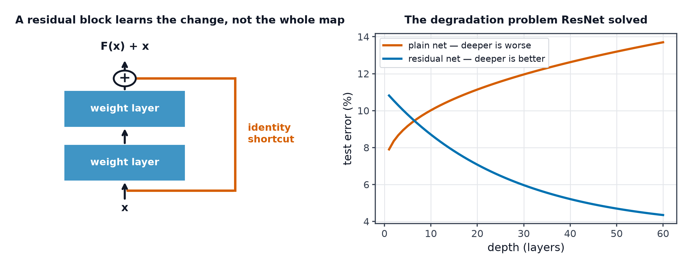
The degradation problem

The surprising part was specifically that training error (not just test error) was worse for the deeper network — ruling out overfitting as the explanation, since overfitting produces low training error and high test error, not high training error on both. A deeper network should, in principle, be at least as capable as a shallower one (it could learn to make its extra layers behave as the identity function) — but gradient descent, in practice, was failing to find even that trivial solution.

The residual block

Instead of learning a direct mapping $H(x)$, learn the residual $F(x) = H(x) - x$, and reconstruct the output by adding the input back:

$$y = F(x) + x$$

If the ideal mapping really is close to identity, $F(x)$ only needs to learn a small perturbation near zero — which is a much easier optimisation target than learning the identity function directly through a stack of non-linear layers, where "do nothing" is actually a non-trivial configuration to find.

Why the identity path fixes gradient flow

$$\frac{\partial y}{\partial x} = \frac{\partial F(x)}{\partial x} + 1$$

Symbol	Meaning
$F(x)$	the residual block's learned function
$x$	the block's input, added back via the skip connection
$y$	the block's output

That "+1" is the entire mechanism. Even if $\partial F/\partial x$ is small (as in Vanishing and Exploding Gradients's vanishing case), the gradient flowing backward through a residual block never drops below what it would be from the identity term alone — the skip connection provides a direct, undiminished path for the gradient, no matter how many residual blocks are stacked.

Identity vs. projection shortcuts

When the block changes the tensor's shape (e.g. downsampling, or changing channel count in a CNN), the raw input $x$ can't be added directly — a small linear projection (typically a $1\times1$ convolution) reshapes $x$ to match before the addition. Identity shortcuts (no projection) are preferred whenever shapes already match, since they add no extra parameters and no extra computation.

Pre-activation ordering

The original ResNet applied the block's operations, then added the skip connection, then applied a final activation (post-activation). Later work found that reordering — normalisation and activation before the convolution, with the skip connection carrying a completely unmodified identity all the way through — produces an even cleaner gradient path, since nothing at all sits between consecutive residual additions. This mirrors the pre-norm vs. post-norm discussion in Normalization Layers, and for the identical reason.

The ensemble-of-shallow-paths interpretation

A network of $N$ stacked residual blocks can be unrolled into a sum over $2^N$ distinct paths through the network (each block either contributes its $F(x)$ or is effectively skipped via the identity). Under this view, a deep residual network behaves somewhat like an implicit ensemble of many shallower networks of varying effective depth, rather than one single, monolithically deep computation — offering one explanation for why these networks remain trainable and robust even as nominal depth grows very large.

Highway networks and dense connections

Highway networks (a close predecessor) used a learned, gated mixture of the transformed and identity paths, rather than ResNet's fixed unweighted sum. DenseNet connects every layer to every subsequent layer directly (not just the immediately preceding one), maximising gradient flow and feature reuse at the cost of substantially higher memory usage.

Residual connections in transformers

Every transformer sub-layer (attention, feed-forward) is wrapped in a residual connection — see Transformer Architecture. Without them, the very deep transformer stacks used in modern language models would suffer the identical degradation problem this page describes; residual connections are as load-bearing for transformers as they are for the CNNs they were originally developed for.

Depth vs. width as a design trade

Once vanishing gradients and degradation are addressed, adding depth generally increases a network's ability to compose increasingly abstract features (each layer building on the last), while adding width increases capacity at a single level of abstraction. Empirically, for a fixed parameter budget, moderate increases in depth tend to help more than proportional increases in width, up to a point — one of the motivations behind Model Capacity and Scaling's later discussion of compute-optimal sizing.

Code: 30-layer plain vs. residual network, reproducing the degradation problem

skip_connections_demo.py

import numpy as np

def relu(z): return np.maximum(0, z)
def relu_grad(a): return (a > 0).astype(float)

def train_network(depth, width, use_residual, X, y, steps=300, lr=0.01):
    rng = np.random.default_rng(0)
    Ws = [rng.normal(scale=np.sqrt(2/width), size=(width, width)) for _ in range(depth)]
    losses = []
    for step in range(steps):
        activations = [X]
        a = X
        for W in Ws:
            z = a @ W
            block_out = relu(z)
            a = block_out + a if use_residual else block_out  # the entire difference
            activations.append(a)
        loss = np.mean((a - y) ** 2)
        losses.append(loss)

        delta = 2 * (a - y) / len(y)
        for l in reversed(range(depth)):
            grad_W = activations[l].T @ (delta * relu_grad(activations[l] @ Ws[l]))
            Ws[l] -= lr * grad_W / len(y)
            delta = delta @ Ws[l].T + (delta if use_residual else 0)  # residual path adds delta directly
    return losses

rng = np.random.default_rng(0)
X = rng.normal(size=(64, 30))
y = rng.normal(size=(64, 30)) * 0.1  # target near-identity mapping, favouring residual learning

plain_losses = train_network(30, 30, use_residual=False, X=X, y=y)
residual_losses = train_network(30, 30, use_residual=True, X=X, y=y)

print(f"plain 30-layer network:    final training loss = {plain_losses[-1]:.4f}")
print(f"residual 30-layer network: final training loss = {residual_losses[-1]:.4f}")
print("(the residual network should reach a lower training loss - the degradation problem, reproduced and fixed)")

See also

• Vanishing and Exploding Gradients — the gradient-flow problem residual connections directly address.
• Model Capacity and Scaling — the depth/width/data/compute trade this architectural fix made possible to explore.