Weight Initialization

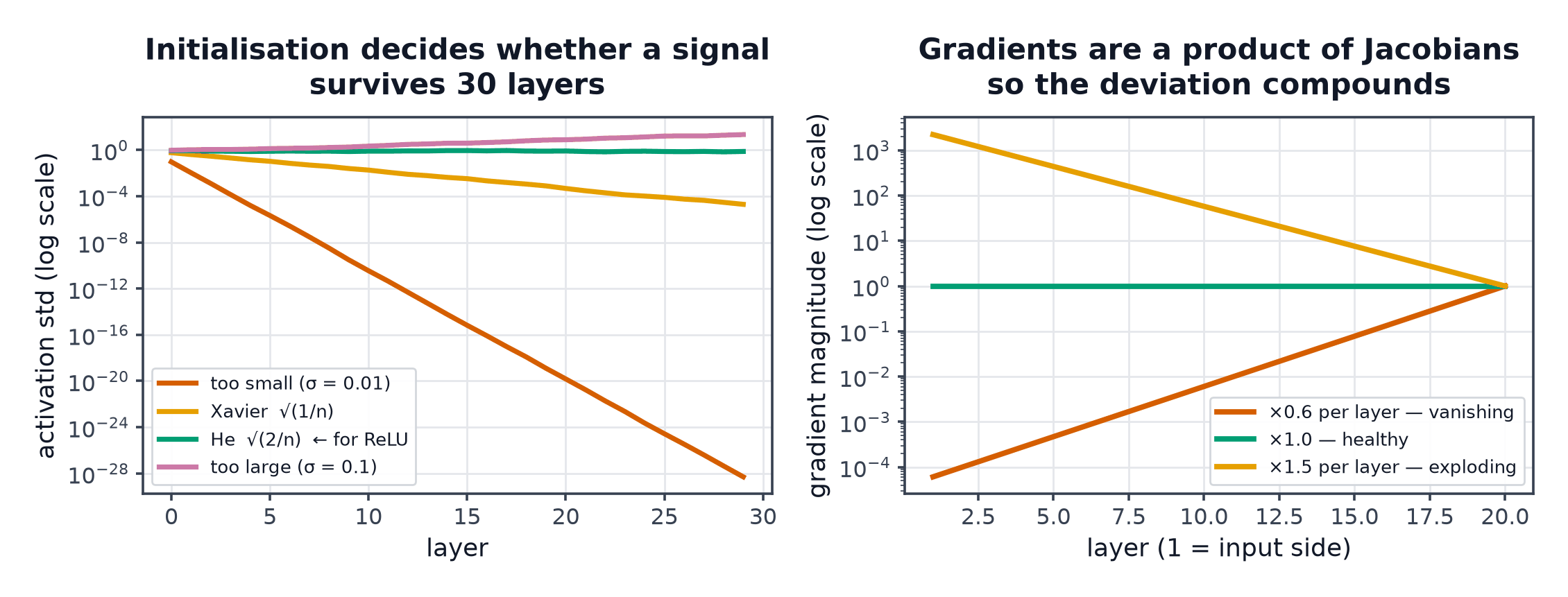
Before the first gradient is ever computed, a choice has already been made that decides whether training has any chance of working: how the weights start. Get it wrong and the signal either dies (shrinks to zero within a few layers) or explodes (grows without bound) before a single useful gradient update happens.

Key idea

Initialise so that activation variance is preserved layer to layer — too small and the signal dies, too large and it explodes.

Initialisation scale decides whether a signal survives depth at all. He initialisation (√(2/n)) holds the activation variance roughly constant through thirty ReLU layers; being off by a constant factor collapses or explodes it exponentially.

Why zeros fail

If every weight starts at zero, every unit in a layer computes the identical output (zero), receives the identical gradient, and updates identically forever — a symmetry that is never broken. Every unit in a layer stays a perfect copy of every other unit for the entire course of training, which means a layer with 1000 units effectively behaves like a layer with 1 unit. This is provable directly: if $W$ is all zeros, $z = Wx = 0$ regardless of $x$, and the gradient with respect to every row of $W$ is identical by symmetry.

Why large random values fail

If weights are drawn from a wide distribution (e.g. $\mathcal{N}(0, 1)$) and the network is even moderately deep, the pre-activations $z^{[l]}$ grow in magnitude with each layer (each layer's output variance multiplies by roughly the previous layer's variance times the number of inputs) — quickly pushing sigmoid/tanh units into their saturated regions (Activation Functions), where the derivative is near zero and gradients vanish despite large activations.

The variance-preservation argument

The fix: choose the initial weight variance so that the variance of activations neither grows nor shrinks as it passes through each layer. For a layer with $n_{\text{in}}$ inputs, if weights are drawn i.i.d. with variance $\text{Var}(W)$, then (under simplifying independence assumptions) the pre-activation variance is approximately:

$$\text{Var}(z) \approx n_{\text{in}} \cdot \text{Var}(W) \cdot \text{Var}(x)$$

Setting $\text{Var}(z) = \text{Var}(x)$ requires $\text{Var}(W) = 1/n_{\text{in}}$.

Xavier/Glorot initialization

For sigmoid/tanh (roughly linear near zero, and needing to preserve variance in both the forward and backward pass), Xavier initialisation balances fan-in and fan-out:

$$\text{Var}(W) = \frac{2}{n_{\text{in}} + n_{\text{out}}}$$

He/Kaiming initialization

ReLU zeros out roughly half its inputs (everything negative), halving the variance that survives each layer relative to a linear unit. He initialisation compensates by doubling the target variance:

$$\text{Var}(W) = \frac{2}{n_{\text{in}}}$$

Symbol	Meaning
$n_{\text{in}}, n_{\text{out}}$	number of input/output units of the layer
$\text{Var}(W)$	target variance for weight initialisation

Why the factor of 2 differs

Xavier assumes a roughly-linear activation preserving all variance; He assumes ReLU, which discards half the variance by zeroing negative inputs, so it needs twice the variance to compensate and still preserve the total signal magnitude — the factor of 2 is not arbitrary, it's derived directly from ReLU's specific behaviour.

Uniform vs. normal variants

Both Xavier and He initialisation are commonly implemented as either a normal distribution with the target variance, or a uniform distribution scaled to match the same variance — the choice rarely matters much in practice, since both preserve the same first two moments.

Bias initialisation

Typically initialised to zero — biases don't participate in the multiplicative variance-scaling argument above the way weights do, since they add a constant rather than scaling the input.

Initialisation for embeddings and the output layer

Embedding tables (Word Embeddings) are typically initialised with a small-variance normal distribution, since they start with no learned structure at all. The final output layer is sometimes initialised specially to set a sensible output prior — for instance, initialising a classifier's final bias to reflect known class frequencies, so the untrained network's initial predictions aren't wildly miscalibrated before any training has occurred.

What normalisation layers changed

Normalization Layers (BatchNorm, LayerNorm) explicitly re-normalise activations at every layer during training, which substantially reduces sensitivity to the initial variance choice — initialisation still matters (a catastrophically bad start can still fail to train), but the strict variance-preservation argument above matters somewhat less in networks that include normalisation layers throughout.

PyTorch defaults, and when to override

PyTorch's built-in layers (nn.Linear, nn.Conv2d) use a variant of He/Kaiming initialisation by default — appropriate for ReLU-family networks out of the box. Override explicitly when using an unusual activation, when the loss stalls immediately at the start of training (a classic initialisation symptom, covered in Debugging Neural Networks), or when following a published architecture with a documented custom initialisation scheme.

Code: three initialisation schemes, activation histograms per layer

weight_init_demo.py

import numpy as np
import matplotlib.pyplot as plt

def relu(z): return np.maximum(0, z)

def forward_with_init(X, n_layers, n_units, init_scheme, rng):
    a = X
    activations_per_layer = []
    for _ in range(n_layers):
        n_in = a.shape[1]
        if init_scheme == "zeros":
            W = np.zeros((n_in, n_units))
        elif init_scheme == "large_random":
            W = rng.normal(scale=1.0, size=(n_in, n_units))
        elif init_scheme == "he":
            W = rng.normal(scale=np.sqrt(2 / n_in), size=(n_in, n_units))
        a = relu(a @ W)
        activations_per_layer.append(a.copy())
    return activations_per_layer

rng = np.random.default_rng(0)
X = rng.normal(size=(500, 50))

fig, axes = plt.subplots(3, 5, figsize=(18, 8))
for row, scheme in enumerate(["zeros", "large_random", "he"]):
    layers = forward_with_init(X, n_layers=10, n_units=50, init_scheme=scheme, rng=np.random.default_rng(0))
    for col, layer_idx in enumerate([0, 2, 4, 6, 9]):
        axes[row, col].hist(layers[layer_idx].ravel(), bins=30)
        axes[row, col].set_title(f"{scheme}, layer {layer_idx+1}")
        if scheme == "zeros":
            axes[row, col].set_xlim(-0.01, 0.01)
plt.savefig("weight_init_histograms.png")

for scheme in ["zeros", "large_random", "he"]:
    layers = forward_with_init(X, n_layers=10, n_units=50, init_scheme=scheme, rng=np.random.default_rng(0))
    print(f"{scheme:15s}: final-layer activation std = {layers[-1].std():.6f}")

Zeros should show every unit collapsed to identically 0; large random should show variance exploding or activations saturating heavily by the later layers; He should show activation standard deviation holding roughly steady across all 10 layers — the variance-preservation argument confirmed directly.

See also

• Vanishing and Exploding Gradients — the training-time consequence of getting this wrong.
• Normalization Layers — the technique that reduces sensitivity to this choice.