Bias-Variance Tradeoff

A model can be wrong in exactly two ways: it can be too simple to capture the real pattern (bias), or too sensitive to the particular training sample it happened to see (variance). Diagnosing which one you're facing tells you whether to add capacity or add data — the two most common fixes are not interchangeable.

Key idea

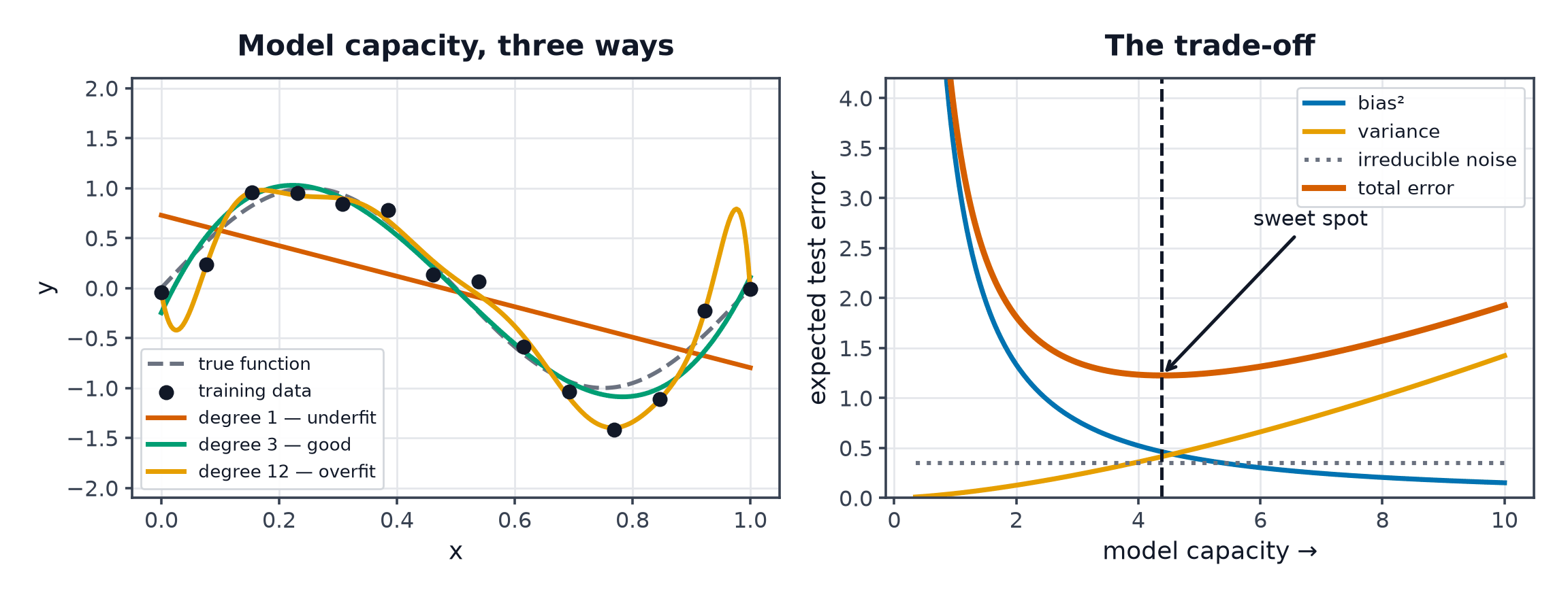
Expected error decomposes into bias squared, variance, and irreducible noise — diagnosis tells you whether to add capacity or add data.

Left, the same 14 points fitted at three capacities — the degree-12 curve chases noise at the edges. Right, the decomposition: total error is a U because bias falls and variance rises, and the irreducible noise floor never moves.

The decomposition, derived

For a model $\hat f$ trained on a random sample, predicting at a fixed point $x$ with true value $y = f(x) + \epsilon$ (noise $\epsilon$, $\mathbb{E}[\epsilon]=0$, $\text{Var}(\epsilon) = \sigma^2$):

$$\mathbb{E}\big[(y - \hat f(x))^2\big] = \underbrace{\big(\mathbb{E}[\hat f(x)] - f(x)\big)^2}_{\text{Bias}^2} + \underbrace{\text{Var}(\hat f(x))}_{\text{Variance}} + \underbrace{\sigma^2}_{\text{irreducible}}$$

Symbol	Meaning
$f(x)$	the true underlying function
$\hat f(x)$	the model's prediction, itself a random variable (depends on the training sample)
$\text{Bias}(\hat f)$	systematic gap between the model's average prediction and the truth
$\text{Var}(\hat f)$	how much the prediction swings across different training samples
$\sigma^2$	noise inherent to the data, no model can remove it

High bias in practice (underfitting)

A linear model fit to a curved relationship has high bias: no matter how much data you give it, it cannot represent the curve, so both training and test error stay high and close together.

High variance in practice (overfitting)

A very deep decision tree fit to a small dataset has high variance: it fits the training data almost perfectly (low training error) but a different training sample would produce a wildly different tree, and test error is much worse than training error.

Irreducible error

$\sigma^2$ is the noise floor — no model, however good, can predict past it. It sets a hard limit on achievable performance; chasing improvements below this floor is chasing noise.

Learning curves

A learning curve plots training and validation error against training-set size.

• High bias: both curves converge to a high error, close together — more data won't help.
• High variance: a large gap between training (low) and validation (higher) error that narrows as training size grows — more data helps directly.

Diagnosis table

Symptom	Cause	Fix
Both train and validation error high, similar	high bias	more capacity, better features, less regularisation
Train error low, validation error much higher	high variance	more data, regularisation, less capacity, ensembling
Both errors low	good fit	ship it

Ensembles as variance reduction, boosting as bias reduction

Averaging many independent high-variance models (bagging, Random Forests) cancels out their individual fluctuations, reducing variance without increasing bias. Boosting (Gradient Boosting) instead sequentially fits residual errors, reducing bias by adding capacity where the current ensemble is systematically wrong.

The modern caveat: double descent

The classical U-shaped curve (error decreases, then increases, as capacity grows) assumed models stop at the point of perfectly fitting the training data. Modern over-parameterised networks continue past that point — and test error can descend again after an initial rise near the interpolation threshold, producing a "double descent" curve. The classical bias-variance story is not wrong, but it's incomplete for models with far more parameters than training examples. Full treatment in Model Capacity and Scaling.

Code: three polynomial degrees, all three regimes

bias_variance_demo.py

import numpy as np
from sklearn.pipeline import make_pipeline
from sklearn.preprocessing import PolynomialFeatures
from sklearn.linear_model import LinearRegression
from sklearn.model_selection import train_test_split, learning_curve

rng = np.random.default_rng(0)
X = rng.uniform(-3, 3, size=(300, 1))
y = 0.5 * X[:, 0] ** 2 - X[:, 0] + rng.normal(scale=1.0, size=300)

X_train, X_test, y_train, y_test = train_test_split(X, y, test_size=0.3, random_state=0)

for degree in [1, 4, 15]:
    model = make_pipeline(PolynomialFeatures(degree), LinearRegression())
    model.fit(X_train, y_train)
    train_err = np.mean((model.predict(X_train) - y_train) ** 2)
    test_err = np.mean((model.predict(X_test) - y_test) ** 2)
    label = {1: "underfits (high bias)", 4: "good fit", 15: "overfits (high variance)"}[degree]
    print(f"degree={degree:2d} ({label:22s}) train_mse={train_err:.3f}  test_mse={test_err:.3f}")

# --- Learning curve for the overfitting degree-15 model ---
model = make_pipeline(PolynomialFeatures(15), LinearRegression())
train_sizes, train_scores, val_scores = learning_curve(
    model, X, y, train_sizes=np.linspace(0.1, 1.0, 5), scoring="neg_mean_squared_error"
)
print("train sizes:", train_sizes)
print("train MSE:", -train_scores.mean(axis=1))
print("val MSE:  ", -val_scores.mean(axis=1))

Degree 1 shows both errors high and close (bias); degree 15 shows a large train/test gap (variance); degree 4 lands closest to the true quadratic relationship.

See also

• Overfitting and Regularization — the fixes for high variance, in depth.
• Train/Validation/Test Splits — how to actually measure the train/validation gap correctly.