Calculus and Gradients

Training a model is repeated use of one operation: measure the slope of the loss with respect to each parameter, then step in the direction that makes the loss smaller. Every optimiser in this knowledge base — from plain gradient descent to Adam — is a variation on that one move. This page derives the machinery once so later pages can use it without re-deriving it.

Key idea

The gradient points in the direction of steepest ascent, so the negative gradient is the only direction a first-order method ever needs.

The derivative is the slope of the tangent. In more than one dimension the gradient points in the direction of steepest *increase* — which is why gradient descent subtracts it.

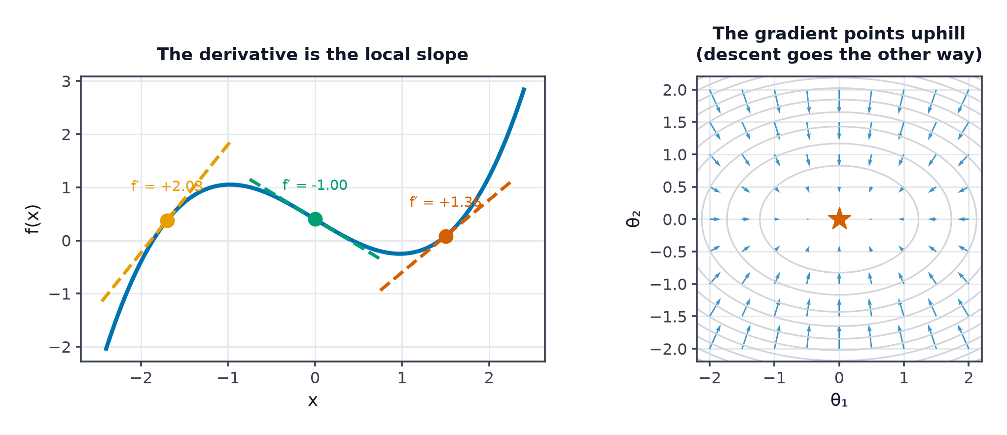
Derivative as local slope

For a scalar function $f(x)$, the derivative $f'(x) = \frac{df}{dx}$ is the instantaneous rate of change — how much $f$ changes for a tiny change in $x$. It is the slope of the tangent line at that point.

Partial derivatives and the gradient

For a function of many variables $f(x_1, \ldots, x_d)$, the partial derivative $\frac{\partial f}{\partial x_i}$ holds every other variable fixed and measures the slope along just $x_i$. Stacking all partial derivatives gives the gradient:

$$\nabla f(x) = \left(\frac{\partial f}{\partial x_1}, \ldots, \frac{\partial f}{\partial x_d}\right)$$

The gradient is a vector pointing in the direction $f$ increases fastest; $-\nabla f$ points in the direction it decreases fastest — the direction every training step moves in.

Symbol	Meaning
$f'(x)$	derivative of a scalar function
$\frac{\partial f}{\partial x_i}$	partial derivative with respect to $x_i$, others held fixed
$\nabla f(x)$	the gradient vector, all partial derivatives stacked

The chain rule

If $y = g(u)$ and $u = h(x)$, then:

$$\frac{dy}{dx} = \frac{dy}{du} \cdot \frac{du}{dx}$$

This single rule, applied repeatedly through a computational graph, is Backpropagation in its entirety — the vector form used there is:

$$\nabla_x f(g(x)) = J_g(x)^\top \nabla_u f(u)$$

where $J_g$ is the Jacobian of $g$.

Jacobian and Hessian

• Jacobian $J$: for a vector-valued function $g: \mathbb{R}^n \to \mathbb{R}^m$, $J_{ij} = \frac{\partial g_i}{\partial x_j}$ — an $m \times n$ matrix of all first derivatives.
• Hessian $H$: for a scalar function, $H_{ij} = \frac{\partial^2 f}{\partial x_i \partial x_j}$ — the matrix of second derivatives, describing curvature.

Convex vs. non-convex surfaces

A convex function has a bowl shape: any local minimum is the global minimum, and gradient descent is guaranteed to find it (with a small enough step size). Neural network losses are almost never convex — they have many local minima, saddle points, and flat regions, which is why deep learning optimisation is an empirical art as much as a theoretical guarantee.

Saddle points

A saddle point has zero gradient but is a minimum along some directions and a maximum along others (the Hessian has both positive and negative eigenvalues). In high dimensions, saddle points vastly outnumber true local minima — it's far more likely for a random critical point to be a saddle than a minimum, because it only takes one bad direction out of thousands to disqualify it as a minimum. This is why "getting stuck in a local minimum" is a less accurate mental model for deep learning than "getting stuck near a saddle point."

Numerical vs. analytic gradients

The analytic gradient is the exact closed-form expression (what the chain rule gives you). The numerical gradient approximates it via finite differences:

$$\frac{\partial f}{\partial x_i} \approx \frac{f(x + \epsilon e_i) - f(x - \epsilon e_i)}{2\epsilon}$$

Numerical gradients are slow (one function evaluation per parameter) and only approximate, but they don't depend on your derivation being correct — which makes them the perfect debugging tool for a hand-derived analytic gradient.

Gradient checking

Compute the analytic gradient, compute the numerical gradient, and compare. If they disagree by more than a small relative tolerance, the analytic derivation (or its code) has a bug. This exact helper is reused in Backpropagation to verify a hand-written backward pass.

Code: analytic gradient, numerical check, reusable helper

gradient_check.py

import numpy as np

def f(x):
    """f(x, y) = (x + y) * x"""
    return (x[0] + x[1]) * x[0]

def analytic_grad(x):
    # df/dx0 = 2*x0 + x1, df/dx1 = x0
    return np.array([2 * x[0] + x[1], x[0]])

def numerical_grad(func, x, eps=1e-5):
    grad = np.zeros_like(x, dtype=float)
    for i in range(len(x)):
        x_plus, x_minus = x.copy(), x.copy()
        x_plus[i] += eps
        x_minus[i] -= eps
        grad[i] = (func(x_plus) - func(x_minus)) / (2 * eps)
    return grad

def gradient_check(func, analytic_fn, x, tol=1e-6):
    """Reused throughout the deep-learning section to verify backward passes."""
    a_grad = analytic_fn(x)
    n_grad = numerical_grad(func, x)
    rel_error = np.linalg.norm(a_grad - n_grad) / (np.linalg.norm(a_grad) + np.linalg.norm(n_grad) + 1e-12)
    print(f"analytic: {a_grad}, numerical: {n_grad}, relative error: {rel_error:.2e}")
    assert rel_error < tol, "gradient check failed"
    return rel_error

x = np.array([2.0, 3.0])
gradient_check(f, analytic_grad, x)

See also

• Gradient Descent — using this gradient to actually train a model.
• Linear Algebra — the vector and matrix notation this page builds on.