Data Preprocessing and Features

Preprocessing decides more of a model's final performance than the choice of algorithm does. It also has to be treated as part of the model, not a one-off step: whatever transformation is applied to training data must travel with the model into production and be fitted only on training data, never on validation or test data (see Train/Validation/Test Splits).

Key idea

Preprocessing is part of the model — it must be fitted on training data only and travel with the model to production.

Numeric scaling

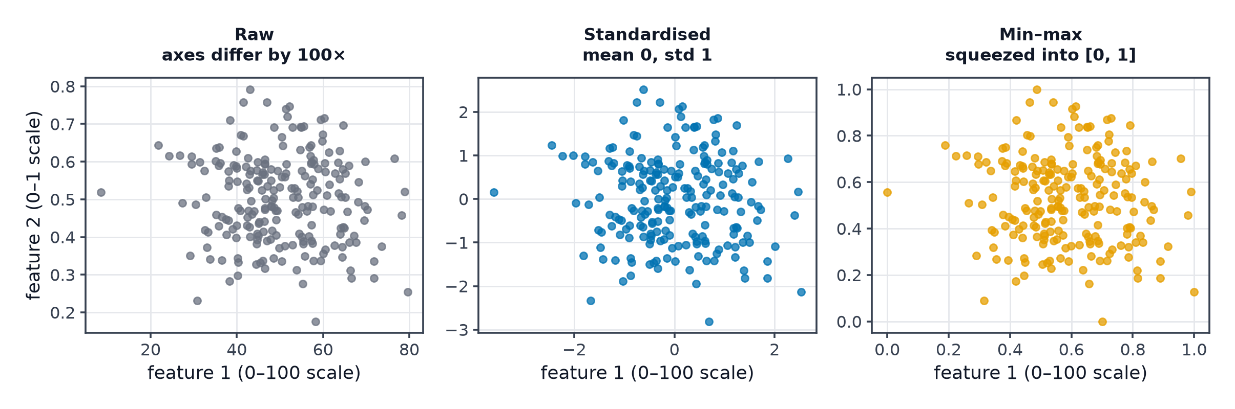
Raw features spanning different ranges dominate any distance- or gradient-based method. Standardisation centres and rescales; min–max squeezes into a fixed interval and is far more sensitive to outliers.

• Standardisation ($z = \frac{x - \mu}{\sigma}$): centres at zero, unit variance. Required for distance-based methods (k-NN), gradient-descent-trained linear models, and neural networks.
• Min-max scaling ($x' = \frac{x - \min}{\max - \min}$): bounds to $[0, 1]$. Sensitive to outliers (a single extreme value compresses everything else).
• Robust scaling (using median and IQR instead of mean and std): tolerant of outliers.

Tree-based models (decision trees, random forests, gradient boosting) are invariant to monotonic transformations of a feature, so scaling doesn't matter for them — a rare exception to "always scale."

Skew and log transforms

Heavily right-skewed features (income, word counts, city population) often benefit from a log transform, which compresses the long tail and makes the distribution closer to Gaussian — useful for linear models and anything assuming roughly normal residuals.

Categorical encoding

• One-hot: one binary column per category. Simple, but explodes in width with high cardinality.
• Ordinal: integer codes, appropriate only when categories have a genuine order (small/medium/large).
• Target encoding: replace a category with the mean target value for that category — powerful, but leaks target information if not done inside cross-validation folds.
• Hashing: map categories to a fixed number of buckets via a hash function — handles unbounded cardinality at the cost of occasional collisions.

Missing values

Options, in order of information preserved: deletion (simplest, discards data), mean/median/mode imputation (simple, can distort variance), model-based imputation (more accurate, more complex), and adding a missingness indicator column alongside the imputed value — because "this value was missing" can itself be predictive (e.g. a skipped survey question correlating with the outcome).

Outliers

Detect (z-score, IQR, or a model like Isolation Forest — see Anomaly Detection), then decide deliberately: clip to a bound, remove, or keep as-is. The right choice depends on whether the outlier is a data error or a genuine (if rare) observation the model should learn from.

Datetime feature extraction

Raw timestamps are rarely useful directly; extract day-of-week, hour, is-weekend, days-since-event, and cyclical encodings (e.g. $\sin, \cos$ of hour-of-day) so that "23:00" and "00:00" are recognised as close rather than maximally distant.

Text and image features

Covered in their own sections: Text Preprocessing and Tokenization for text, Images as Tensors for images.

Interaction and polynomial features

Multiplying two features together (or squaring one) lets a linear model capture relationships it otherwise couldn't express — at the cost of a rapidly growing feature count as you add more interaction terms.

Feature selection

• Filter methods: score each feature independently (correlation, mutual information) before modelling — fast, ignores feature interactions.
• Wrapper methods: repeatedly fit a model on feature subsets and keep the subset with the best validation score — expensive, accounts for interactions.
• Embedded methods: the model itself performs selection during fitting (L1 regularisation zeroing out coefficients, tree-based feature importances).

Pipeline and ColumnTransformer

Fitting a scaler before splitting leaks the test set's mean and variance into training. The result is an optimistic validation score that vanishes in production. Fit on train, apply to test — always in that order.

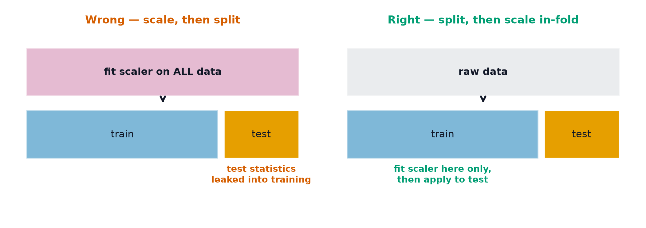
The leak-proof way to combine all of the above: wrap every preprocessing step and the model itself into a single Pipeline, so that calling .fit() inside a single cross-validation fold fits the scaler, encoder, and model only on that fold's training data — nothing from the validation portion ever touches the fitted transformers.

Code: a full ColumnTransformer + Pipeline, and the leak it prevents

preprocessing_pipeline_demo.py

import numpy as np
import pandas as pd
from sklearn.compose import ColumnTransformer
from sklearn.pipeline import Pipeline
from sklearn.preprocessing import StandardScaler, OneHotEncoder
from sklearn.impute import SimpleImputer
from sklearn.linear_model import LogisticRegression
from sklearn.model_selection import cross_val_score, StratifiedKFold

rng = np.random.default_rng(0)
n = 500
df = pd.DataFrame({
    "age": rng.normal(40, 12, n),
    "income": rng.lognormal(mean=10, sigma=1, size=n),
    "city": rng.choice(["NYC", "LA", "Chicago", None], size=n, p=[0.4, 0.3, 0.25, 0.05]),
})
y = (df["age"] > 40).astype(int).values

numeric_features = ["age", "income"]
categorical_features = ["city"]

numeric_pipeline = Pipeline([
    ("impute", SimpleImputer(strategy="median")),
    ("scale", StandardScaler()),
])
categorical_pipeline = Pipeline([
    ("impute", SimpleImputer(strategy="most_frequent")),
    ("onehot", OneHotEncoder(handle_unknown="ignore")),
])

preprocessor = ColumnTransformer([
    ("num", numeric_pipeline, numeric_features),
    ("cat", categorical_pipeline, categorical_features),
])

full_pipeline = Pipeline([("preprocess", preprocessor), ("clf", LogisticRegression())])

# Correct: everything fitted inside each CV fold, no leak
skf = StratifiedKFold(n_splits=5, shuffle=True, random_state=0)
scores = cross_val_score(full_pipeline, df, y, cv=skf, scoring="accuracy")
print("correct pipeline CV accuracy:", scores.mean())

# --- Leaky version: scale on the full dataset BEFORE cross-validation ---
X_num = df[numeric_features].fillna(df[numeric_features].median())
X_scaled_leaked = StandardScaler().fit_transform(X_num)  # sees the whole dataset first
leaky_scores = cross_val_score(LogisticRegression(), X_scaled_leaked, y, cv=skf)
print("leaky (scaled before split) CV accuracy:", leaky_scores.mean())

See also

• Train/Validation/Test Splits — why the Pipeline pattern above is mandatory, not optional.
• Curse of Dimensionality — what happens when one-hot encoding or interaction features push feature count too high.