Evaluation Metrics for Classification

Accuracy is the wrong metric more often than it is the right one. A model that predicts "healthy" for every patient in a dataset where 99% of patients are healthy scores 99% accuracy while being completely useless. Picking the right metric means picking it from the cost of each error type, not from convention.

Key idea

Pick the metric from the cost of each error type, not from convention.

Every classification metric is a ratio computed from these four cells. With 10 % positives, predicting 'negative' always would score 90 % accuracy while catching nothing.

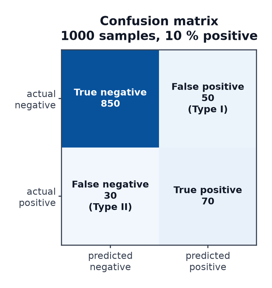
The confusion matrix

	Predicted positive	Predicted negative
Actually positive	True positive (TP)	False negative (FN)
Actually negative	False positive (FP)	True negative (TN)

Every classification metric below is computed from these four counts.

Accuracy and the imbalance trap

$$\text{Accuracy} = \frac{TP + TN}{TP + TN + FP + FN}$$

On a 99/1 imbalanced dataset, predicting the majority class every time scores 99% accuracy while catching zero of the minority class. Accuracy is only trustworthy when classes are roughly balanced and both error types cost about the same.

Precision and recall

$$\text{Precision} = \frac{TP}{TP + FP}, \qquad \text{Recall} = \frac{TP}{TP + FN}$$

Precision answers "of everything I flagged positive, how much was actually positive?" — it protects against false alarms. Recall answers "of everything actually positive, how much did I catch?" — it protects against missed cases. A spam filter favours precision (don't flag real mail); a cancer screen favours recall (don't miss real cases).

F1 and F-beta

$$F_1 = \frac{2 \cdot \text{Precision} \cdot \text{Recall}}{\text{Precision} + \text{Recall}}, \qquad F_\beta = (1+\beta^2) \frac{\text{Precision} \cdot \text{Recall}}{\beta^2 \cdot \text{Precision} + \text{Recall}}$$

$F_1$ is the harmonic mean of precision and recall — punishing a large gap between them more than an arithmetic mean would. $F_\beta$ with $\beta > 1$ weights recall more heavily; $\beta < 1$ weights precision more heavily.

Specificity and sensitivity

$$\text{Sensitivity} = \text{Recall} = \frac{TP}{TP+FN}, \qquad \text{Specificity} = \frac{TN}{TN+FP}$$

Specificity is recall's mirror on the negative class — "of everything actually negative, how much did I correctly call negative?"

The threshold is a choice

The model produces a score; you choose the threshold. Moving it left catches more positives at the cost of more false alarms. Where you put it is a business decision, not a modelling one.

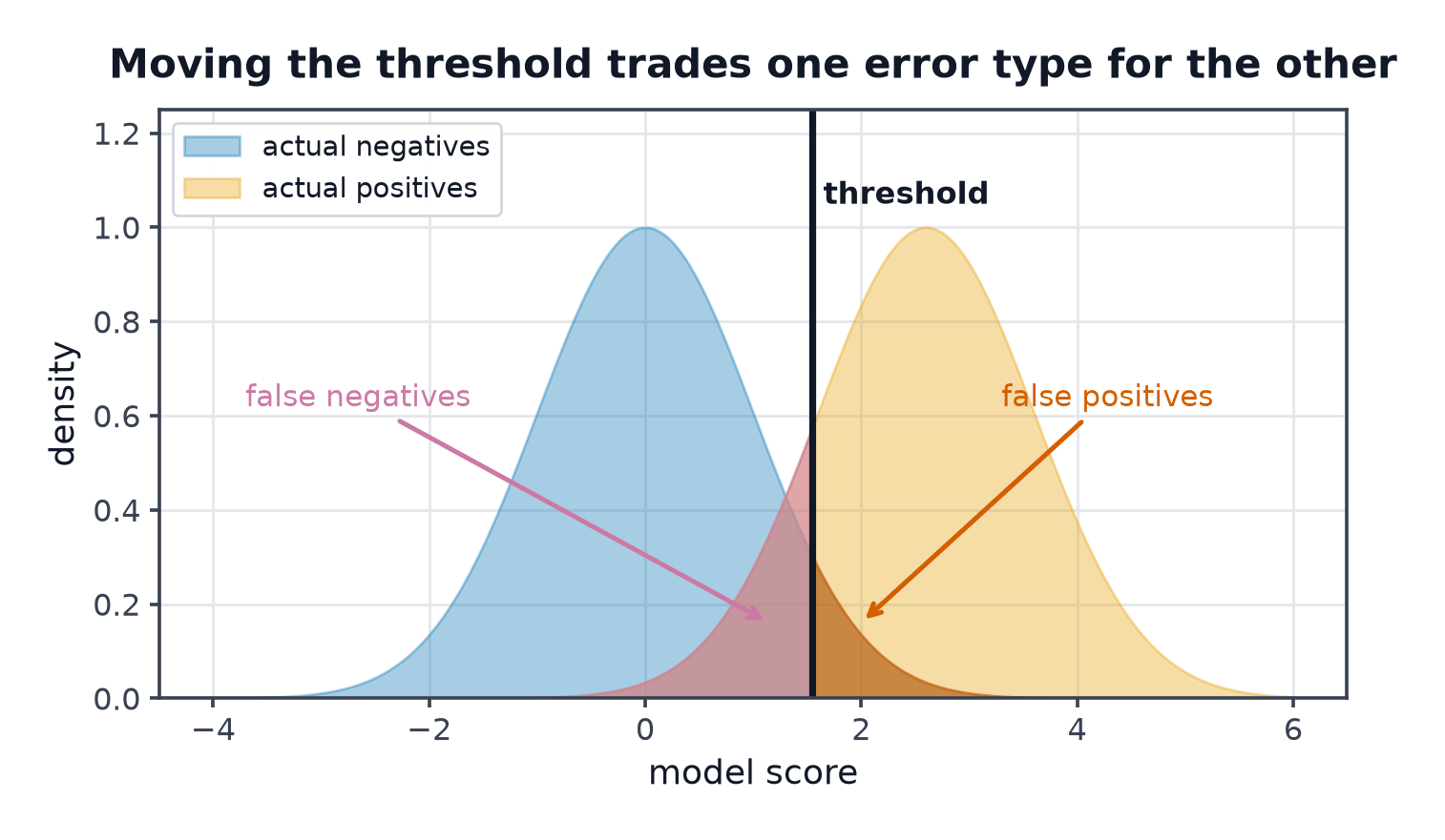
Most classifiers output a probability, not a hard label; the 0.5 cutoff is a convention, not a law. Moving the threshold trades precision for recall in a predictable, continuous way — the right threshold comes from the actual cost of each error type, decided during problem framing (The ML Workflow), not left at the library default.

ROC curve and AUC

The same model on the same imbalanced data. ROC looks strong because true negatives dominate the false-positive rate; the precision–recall curve, which ignores true negatives, shows the real weakness. On imbalanced problems, trust the right-hand plot.

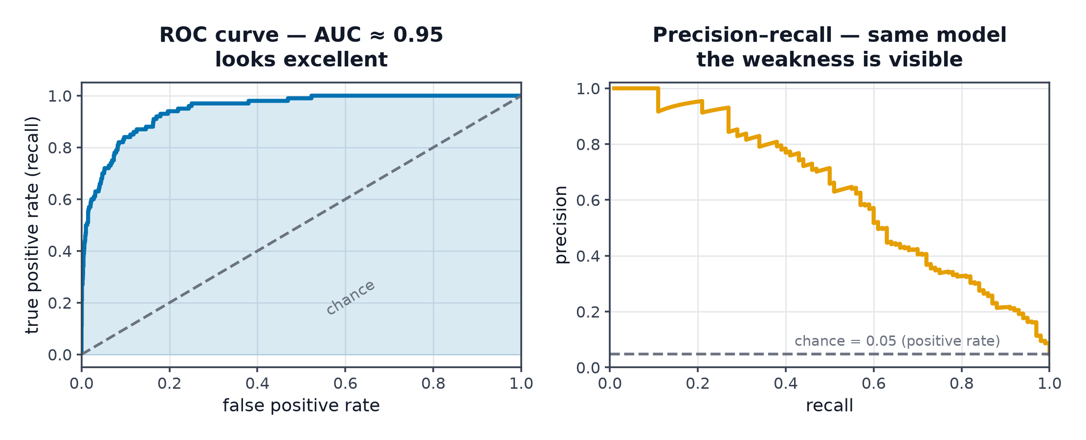
The ROC curve plots true positive rate (recall) against false positive rate ($FPR = \frac{FP}{FP+TN}$) as the threshold sweeps from 0 to 1. AUC (area under this curve) summarises performance across all thresholds at once — 0.5 is random guessing, 1.0 is perfect separation.

Precision-recall curve

Plots precision against recall as the threshold sweeps. On heavily imbalanced data, the PR curve is more informative than ROC — because ROC's false positive rate is normalised by the (huge) number of true negatives, it can look deceptively good even when precision is terrible, while the PR curve exposes that directly.

Multi-class averaging

• Micro: pool all TP/FP/FN across classes, then compute — dominated by the largest classes.
• Macro: compute per-class, then average unweighted — every class counts equally, regardless of size.
• Weighted: average per-class scores weighted by class frequency.

Calibration

A model is well-calibrated if, among all predictions with confidence 0.8, roughly 80% are actually correct. A reliability diagram (predicted probability vs. observed frequency, binned) reveals over- or under-confidence — a model can have high accuracy and still be badly calibrated, which matters whenever downstream decisions use the probability itself, not just the label.

Symbol	Meaning
$TP, FP, TN, FN$	true/false positive/negative counts
Precision, Recall	see above
$\beta$	F-beta's weighting between precision and recall

Metric selection table

Which error hurts more?	Reach for
False positives (false alarms costly)	Precision, or a high threshold
False negatives (missed cases costly)	Recall, or a low threshold
Both matter, roughly equally	F1
Comparing models across all thresholds, balanced data	ROC-AUC
Comparing models across all thresholds, imbalanced data	PR-AUC
Decisions depend on the probability itself	Calibration

Code: confusion matrix, curves, threshold sweep

classification_metrics_demo.py

import numpy as np
from sklearn.datasets import make_classification
from sklearn.model_selection import train_test_split
from sklearn.linear_model import LogisticRegression
from sklearn.metrics import (
    confusion_matrix, classification_report, roc_curve, roc_auc_score,
    precision_recall_curve,
)

X, y = make_classification(n_samples=2000, weights=[0.9, 0.1], random_state=0)
X_train, X_test, y_train, y_test = train_test_split(X, y, test_size=0.3, stratify=y, random_state=0)

model = LogisticRegression().fit(X_train, y_train)
probs = model.predict_proba(X_test)[:, 1]
preds = (probs >= 0.5).astype(int)

print(confusion_matrix(y_test, preds))
print(classification_report(y_test, preds))
print("ROC-AUC:", roc_auc_score(y_test, probs))

# --- Sweep the decision threshold ---
print("\nthreshold | precision | recall")
precisions, recalls, thresholds = precision_recall_curve(y_test, probs)
for t in [0.1, 0.3, 0.5, 0.7, 0.9]:
    idx = np.argmin(np.abs(thresholds - t))
    print(f"{t:8.1f}  |  {precisions[idx]:.3f}   |  {recalls[idx]:.3f}")

Lowering the threshold from 0.5 toward 0.1 pushes recall up and precision down, and vice versa raising it toward 0.9 — the table makes that trade concrete rather than abstract.

See also

• Evaluation Metrics for Regression — the equivalent toolkit for continuous targets.
• Imbalanced Data — the full treatment of imbalance this page only introduces.