Gradient Descent

Nearly every model in this knowledge base is trained the same way: compute the gradient of the loss, take a small step in the opposite direction, repeat. The entire difficulty is in choosing how big a step and how much noise to tolerate along the way.

Key idea

Take the negative gradient, scale it by a learning rate, repeat — the entire difficulty is in the scaling and the noise.

The update rule

$$w \leftarrow w - \eta \, \nabla L(w)$$

Symbol	Meaning
$w$	the parameters being optimised
$\eta$	learning rate — how big a step to take
$\nabla L(w)$	gradient of the loss with respect to $w$

Learning rate: too small, too large, just right

The same loss surface and starting point, three learning rates. Too small never arrives in the budget you have; too large diverges. Note the middle path still bends — it descends the steep axis first, then travels the shallow one.

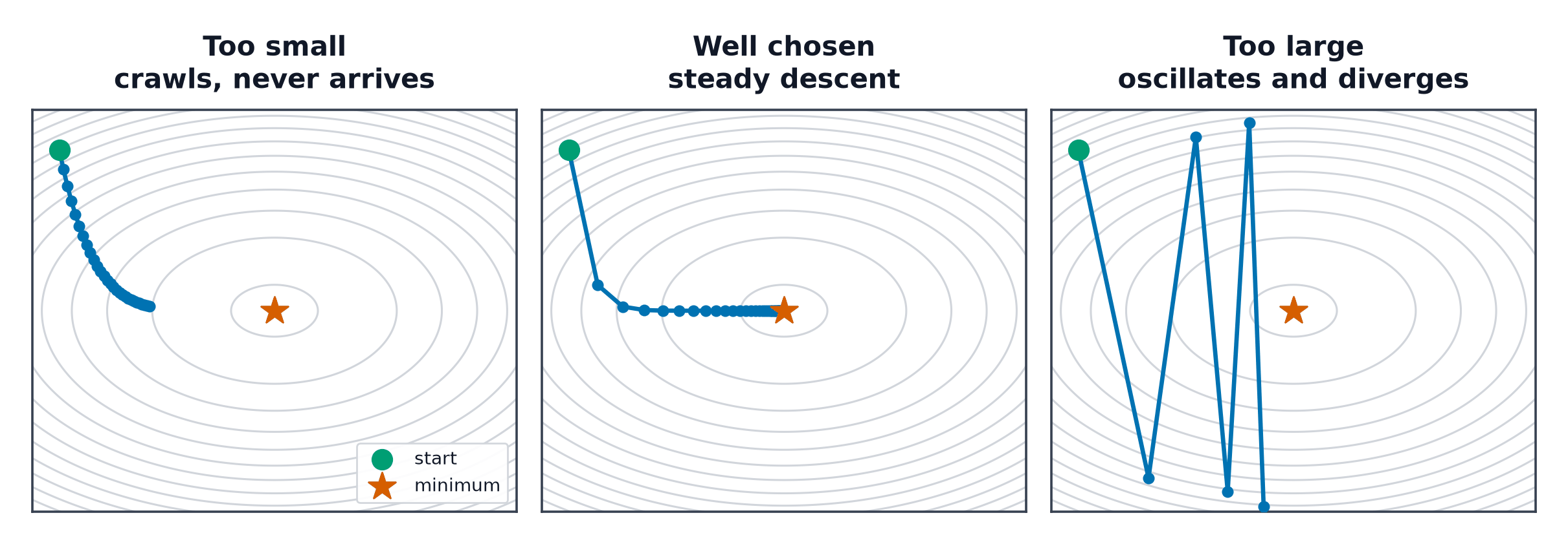
Too small: convergence is correct but painfully slow — thousands of steps to get anywhere. Too large: the update overshoots the minimum, and the loss can oscillate or diverge entirely, sometimes growing without bound. The right learning rate depends on the loss surface's curvature, which is why Learning Rate Schedules exist — a fixed value rarely stays optimal throughout training.

Batch vs. stochastic vs. mini-batch

Gradient noise rises as the batch shrinks. The noise is not purely a cost — it is what lets SGD escape shallow local minima that full-batch descent settles into.

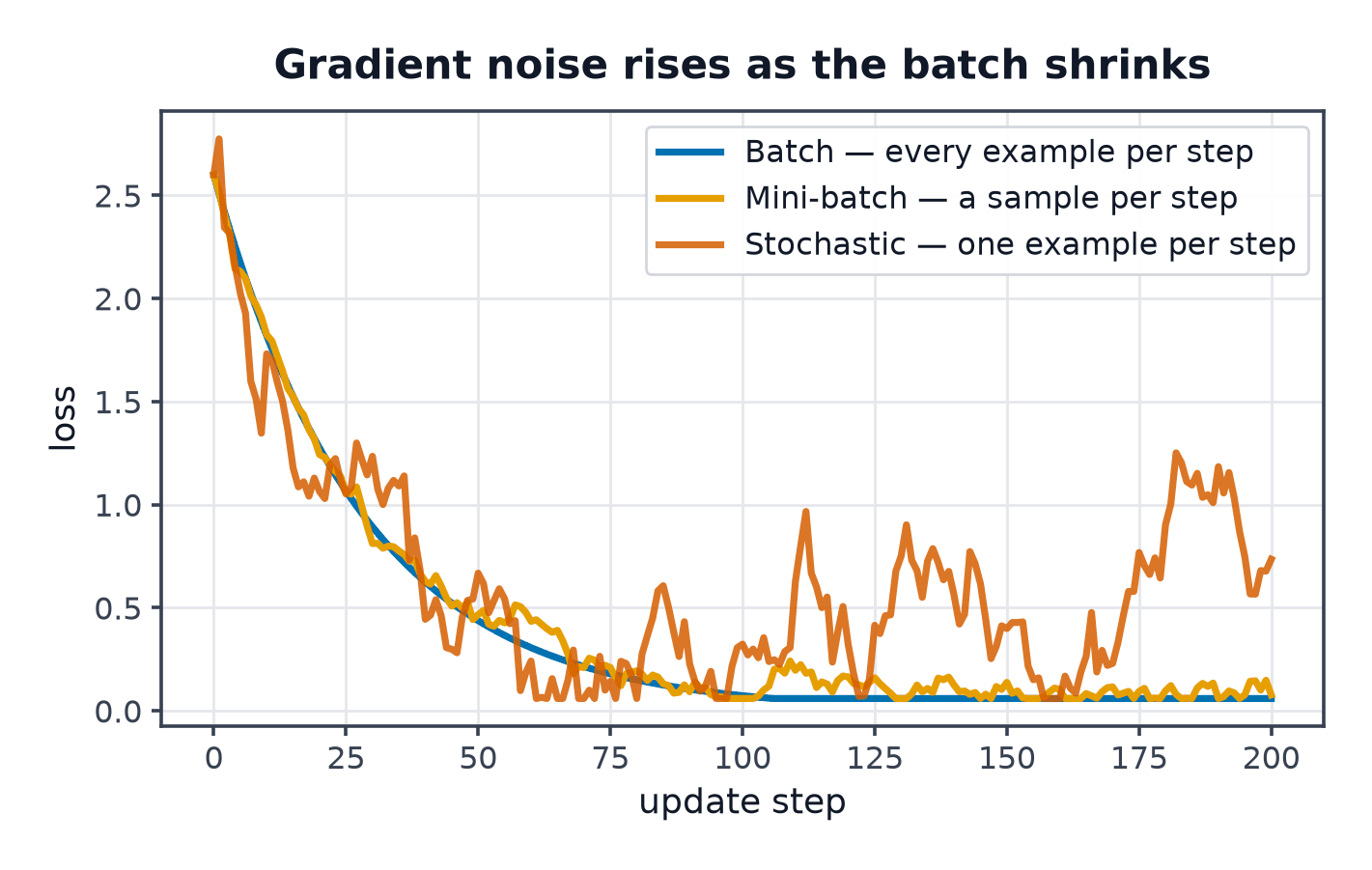
• Batch (full-dataset) gradient descent: compute the exact gradient over every training example before stepping. Correct direction, but one step per full pass over the data — very slow for large datasets.
• Stochastic gradient descent (SGD): estimate the gradient from a single random example. Noisy, but incredibly cheap per step, and the noise itself has a mild regularising effect.
• Mini-batch: estimate the gradient from a small random batch (e.g. 32–256 examples) — the practical default, balancing gradient accuracy against per-step cost and making good use of parallel hardware.

Epochs, steps, batch size

One epoch is one full pass over the training data. One step is one parameter update, using one mini-batch. If the dataset has $n$ examples and batch size is $b$, one epoch contains $\lceil n/b \rceil$ steps.

Convergence on convex vs. non-convex surfaces

On a convex loss, gradient descent with a suitable learning rate provably converges to the global minimum. Neural network losses are non-convex, so no such guarantee holds — but in practice, over-parameterised networks tend to find solutions that generalise well anyway, a phenomenon still not fully explained by theory (see Model Capacity and Scaling).

Local minima, saddles, plateaus

A local minimum has zero gradient and positive curvature in every direction — genuinely stuck. A saddle point has zero gradient but mixed curvature — in high dimensions these dominate (see Calculus and Gradients). A plateau is a flat region with near-zero gradient everywhere — not a minimum, just slow going, which is where momentum helps most.

Momentum, motivated

Plain gradient descent forgets its history at every step. Momentum accumulates a running average of past gradients, so consistent downhill directions accelerate while oscillating directions cancel out:

$$v \leftarrow \beta v + \nabla L(w), \qquad w \leftarrow w - \eta v$$

Think of it as a ball rolling downhill: it picks up speed on a consistent slope and doesn't instantly reverse direction in a narrow ravine, unlike a memoryless step. Full derivation and variants in Optimizers.

Reading a loss curve

Pattern	Likely cause
Steady, smooth decrease	healthy training
Flat from the start	learning rate too small, or a bug (check gradients aren't zero)
Diverging (loss grows)	learning rate too large
Wildly oscillating	learning rate too large, or batch size too small
Decreasing then suddenly spiking	numerical instability, often from an unclipped gradient

When gradient descent is the wrong tool

Some problems have a closed-form solution — linear regression's normal equation solves for the optimum in one step, no iteration required (see Linear Regression). Others are non-differentiable — hard threshold functions, discrete decisions — where gradient descent simply doesn't apply and you need a different search strategy (decision trees split by information gain, not gradients).

Code: hand-written gradient descent, three learning rates, mini-batch

gradient_descent_demo.py

import numpy as np
import matplotlib.pyplot as plt

rng = np.random.default_rng(0)
n, d = 200, 3
X = rng.normal(size=(n, d))
true_w = np.array([2.0, -1.0, 0.5])
y = X @ true_w + rng.normal(scale=0.1, size=n)

def mse_loss(w, X, y):
    return np.mean((X @ w - y) ** 2)

def mse_grad(w, X, y):
    return 2 * X.T @ (X @ w - y) / len(y)

def gradient_descent(X, y, lr, steps=200):
    w = np.zeros(X.shape[1])
    losses = []
    for _ in range(steps):
        losses.append(mse_loss(w, X, y))
        w -= lr * mse_grad(w, X, y)
    return w, losses

# --- Closed-form normal equation, for comparison ---
w_closed_form = np.linalg.pinv(X.T @ X) @ X.T @ y
print("closed-form solution:", w_closed_form)

fig, ax = plt.subplots()
for lr, label in [(0.001, "too small"), (0.05, "healthy"), (0.6, "too large / diverging")]:
    _, losses = gradient_descent(X, y, lr)
    ax.plot(losses, label=f"lr={lr} ({label})")
ax.set_yscale("log")
ax.legend()
plt.savefig("gd_learning_rates.png")

# --- Mini-batch variant ---
def minibatch_gd(X, y, lr, batch_size=32, steps=200, seed=0):
    rng_local = np.random.default_rng(seed)
    w = np.zeros(X.shape[1])
    for _ in range(steps):
        idx = rng_local.choice(len(y), size=batch_size, replace=False)
        w -= lr * mse_grad(w, X[idx], y[idx])
    return w

w_mb = minibatch_gd(X, y, lr=0.05)
print("mini-batch solution:", w_mb, " (true w:", true_w, ")")

See also

• Calculus and Gradients — the derivative machinery this update rule uses.
• Loss Functions — what's actually being minimised.
• Optimizers — momentum, Adam, and everything past plain gradient descent.