Loss Functions

The loss is the only thing the model actually optimises. Every other design choice — architecture, optimiser, regularisation — is in service of minimising this one number. Choose it carelessly and the model will optimise exactly what you asked for, which is often not what you meant.

Key idea

A loss encodes both the task and your assumptions about noise; the metric you report and the loss you train are frequently not the same function.

Squared error punishes outliers quadratically; absolute error does not; Huber is quadratic near zero and linear beyond it. On the right, cross-entropy is unbounded — a confident wrong prediction is penalised without limit.

What makes a valid loss

A loss $L(\hat y, y)$ must be differentiable (or subdifferentiable) with respect to the model's parameters, and it must be minimised exactly when predictions match targets. Accuracy fails the first requirement — it's a step function, flat almost everywhere, with zero useful gradient. This is why classifiers train on cross-entropy but get reported on accuracy.

Regression losses

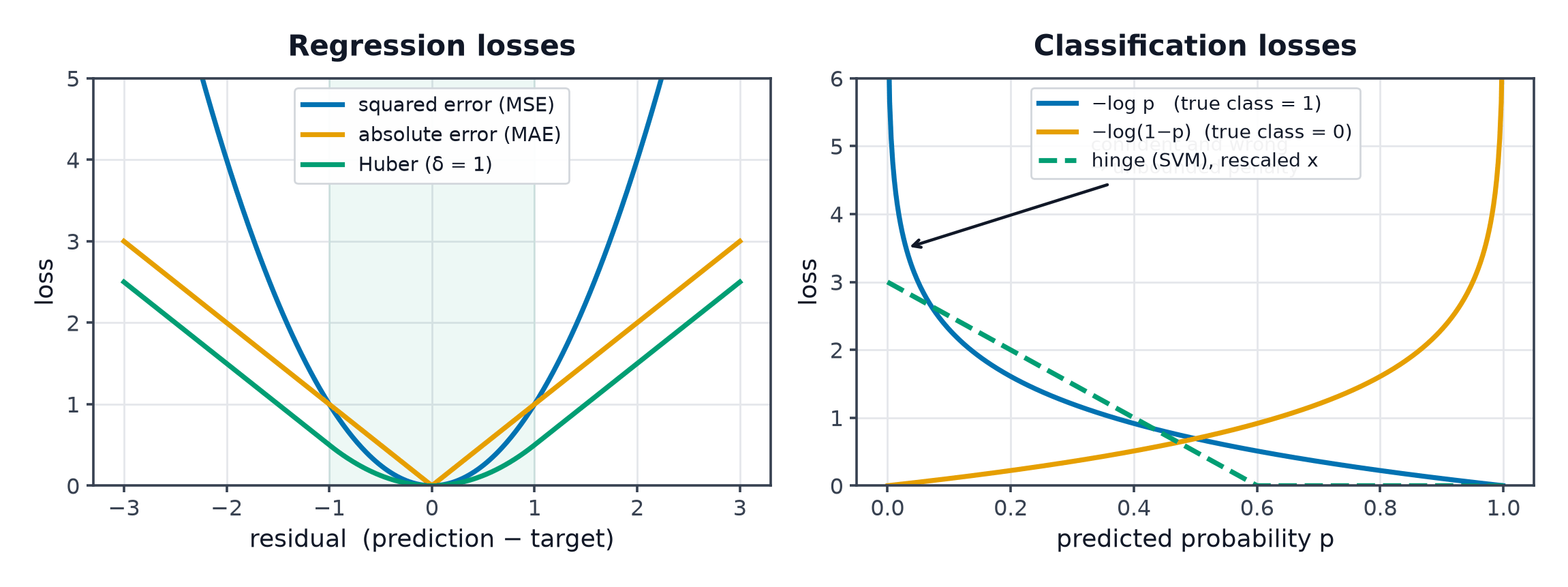
MSE (mean squared error): $L = \frac{1}{n}\sum_i (y_i - \hat y_i)^2$. Penalises large errors quadratically — a single big outlier dominates the loss and pulls the fit toward it.

MAE (mean absolute error): $L = \frac{1}{n}\sum_i |y_i - \hat y_i|$. Penalises all errors linearly — robust to outliers, but has a non-differentiable point at zero error.

Huber loss: quadratic for small errors, linear for large ones, controlled by a threshold $\delta$:

$$L_\delta(r) = \begin{cases} \frac{1}{2}r^2 & |r| \le \delta \\ \delta\left(|r| - \frac{1}{2}\delta\right) & |r| > \delta \end{cases}, \quad r = y - \hat y$$

Huber gets MSE's smoothness near zero and MAE's outlier robustness far from zero.

Classification losses

Binary cross-entropy: $L = -\frac{1}{n}\sum_i \big[y_i \log \hat p_i + (1-y_i)\log(1 - \hat p_i)\big]$, where $\hat p_i$ is the predicted probability of the positive class.

Categorical cross-entropy: $L = -\frac{1}{n}\sum_i \log \hat p_{i, y_i}$ — the negative log-probability the model assigned to the true class.

Why not accuracy: accuracy has zero gradient almost everywhere, so it cannot guide optimisation. Cross-entropy is a smooth surrogate — minimising it tends to also improve accuracy, but the two can diverge (a model can improve cross-entropy by becoming better-calibrated while accuracy stays flat).

Hinge loss

$$L = \max(0, 1 - y \hat f(x)), \quad y \in \{-1, +1\}$$

Zero once a prediction is correct and beyond a margin of confidence; used by Support Vector Machines — it penalises being "barely right," pushing the decision boundary away from training points, not just onto the correct side.

Focal loss

$$L = -\alpha (1 - \hat p)^\gamma \log \hat p$$

A cross-entropy variant that down-weights easy, already-confident examples (via the $(1-\hat p)^\gamma$ term) so the loss focuses on hard, misclassified ones — designed for severe class imbalance (Imbalanced Data).

Ranking and contrastive losses, briefly

Triplet loss and contrastive loss (used in embeddings and metric learning) don't score a single prediction against a single target — they score relative distances between pairs or triplets, pulling similar items together and dissimilar items apart. Covered in depth in Self-Supervised Vision.

Symbol	Meaning
$y_i, \hat y_i$	true and predicted value
$\hat p_i$	predicted probability
$\delta$	Huber's threshold between quadratic and linear regions
$\gamma, \alpha$	focal loss's focusing and balancing parameters

Loss vs. metric

The loss must be differentiable; the metric you report to stakeholders doesn't have to be, and often shouldn't be the same function. You train on cross-entropy but report F1 or AUC because those better reflect the real-world cost of errors (Evaluation Metrics for Classification).

Class weighting

Multiply each example's loss contribution by a weight inversely proportional to its class frequency, so a rare class's mistakes count as much as a common class's:

$$L = \frac{1}{n}\sum_i w_{y_i}\, L_i, \quad w_c = \frac{n}{k \cdot n_c}$$

Selection table

Task	Default loss	Reach for instead when...
Regression	MSE	outliers are common → MAE or Huber
Binary classification	Binary cross-entropy	severe imbalance → focal loss + class weights
Multi-class classification	Categorical cross-entropy	—
Margin-based classification	Hinge loss	SVM-style large-margin boundary desired
Embeddings / similarity	Contrastive / triplet	learning a distance, not a label

Code: every loss, from scratch, verified

loss_functions_demo.py

import numpy as np
from sklearn.metrics import mean_squared_error, mean_absolute_error, log_loss

def mse(y, y_hat):
    return np.mean((y - y_hat) ** 2)

def mae(y, y_hat):
    return np.mean(np.abs(y - y_hat))

def huber(y, y_hat, delta=1.0):
    r = y - y_hat
    is_small = np.abs(r) <= delta
    return np.mean(np.where(is_small, 0.5 * r**2, delta * (np.abs(r) - 0.5 * delta)))

def binary_cross_entropy(y, p_hat, eps=1e-12):
    p_hat = np.clip(p_hat, eps, 1 - eps)
    return -np.mean(y * np.log(p_hat) + (1 - y) * np.log(1 - p_hat))

rng = np.random.default_rng(0)
y_true = rng.normal(size=200)
y_pred = y_true + rng.normal(scale=0.5, size=200)
y_pred_outlier = y_pred.copy()
y_pred_outlier[0] += 50  # inject one huge outlier

print("MSE (clean):", mse(y_true, y_pred), " sklearn:", mean_squared_error(y_true, y_pred))
print("MAE (clean):", mae(y_true, y_pred), " sklearn:", mean_absolute_error(y_true, y_pred))
print("MSE with outlier:", mse(y_true, y_pred_outlier))
print("MAE with outlier:", mae(y_true, y_pred_outlier), "  <- barely moved, unlike MSE")
print("Huber with outlier:", huber(y_true, y_pred_outlier))

labels = rng.integers(0, 2, size=100)
probs = np.clip(labels + rng.normal(scale=0.3, size=100), 0.01, 0.99)
print("BCE:", binary_cross_entropy(labels, probs), " sklearn:", log_loss(labels, probs))

The outlier test is the point: MSE roughly doubles when one point moves 50 units away, while MAE barely changes — direct evidence of the two losses' different tolerance for outliers.

See also

• Information Theory — the entropy/KL machinery cross-entropy is built from.
• Gradient Descent — how these losses are actually minimised.
• Evaluation Metrics for Classification — the metrics reported instead of the loss trained.